Local search and the hill climbing algorithm

The scope of local search methods goes beyond the “classical” approach of seeking the shortest path to a goal state in an observable, deterministic, and discrete environment. In local search, the path is irrelevant. It operates on the current node only (with a complete-state formulation) rather than on multiple paths simultaneously (no frontier is involved).

Local search looks for the extrema of an objective function in a non-systematic way, but it is complete, as it always finds reasonable solutions if they exist. Thus, it is adequate for optimisation problems. However, it is only guaranteed to be optimal if one single (global) extremum exists. Otherwise, it will get stuck on any of the local extrema.

Hill climbing in detail

Hill climbing, aka steepest-ascent, is a greedy approach that operates in a loop that continually moves in the direction of increasing value, that is, uphill, until it reaches a “peak” (i.e., a maximum) where no neighbour shows a higher value, see Figure 1.

Figure 1. Hill climbing applied on a one-dimensional state-space landscape described by an example objective function .

Hill climbing on a state-space landscape
Hill climbing on a state-space landscape.

Hill climbing gets stuck at local maxima, plateaus and ridges. In case of failure (i.e., not reaching the global maximum), you may restart the process with a different initial value. Hill climbing displays a unit space complexity (i.e., the current state) and a linear time complexity (with respect to the number of neighbouring states). Figure 2 implements this algorithm on a one-dimensional state-space.

Figure 2. Hill climbing algorithm.

-- Hill climbing algorithm.
--
-- PRE:
-- problem - must be an array of costs, index indicates state (table).
-- start - must be the starting state index (number).
--
-- POST:
-- solution - is the solution state (number).


function hill_climbing(problem, start)
  local current = start
  local neighbour
  local change
  while (true) do
    if (current == 1) then
      neighbour, change = eval_right(problem, current)
    elseif (current == #problem) then
      neighbour, change = eval_left(problem, current)
    else
      neighbour, change = eval_left(problem, current)
      if (change == false) then
        neighbour, change = eval_right(problem, current)
      end
    end
    if (change) then
      current = neighbour
    else
      return current
    end
  end
end

function eval_left(problem, current)
  if (problem[current - 1] > problem[current]) then
    return current - 1, true
  else
    return current, false
  end
end

function eval_right(problem, current)
  if (problem[current + 1] > problem[current]) then
    return current + 1, true
  else
    return current, false
  end
end

Despite the (arguably) poor performance of hill climbing to find the global maximum, it is an intuitive algorithm that provides a lot of insight into the nature of the optimisation problems and a rule of thumb to solve them. The next posts will address this lack of skill and suggest more powerful optimisation routines. Stay tuned!

The recursive best-first search algorithm

The recursive best-first search (RBFS) algorithm is a simple recursive algorithm that attempts to mimic the operation of A-star search (i.e., the standard best-first search with an evaluation function that adds up the path cost and the heuristic), but using only linear space (instead of showing an exponential space complexity). The structure of RBFS is similar to that of recursive depth-first search (a tree-search version), but rather than continuing indefinitely down the current path, it uses an evaluation limit to keep track of the best alternative path available from any ancestor of the current node, see Figure 1.

Figure 1. RBFS applied on the graphical map of Germany, from Frankfurt to München.

RBFS applied on the graphical map of Germany
RBFS applied on the graphical map of Germany.

RBFS is robust and optimal (if the heuristic is admissible), but it still suffers from excessive node regeneration due to its low memory profile, which entails a long processing time. Given enough time, though, it can solve problems that A-star cannot solve because it runs out of memory.

Figure 2. Recursive best-first search algorithm.

-- Recursive best-first search algorithm.
--
-- PRE:
-- problem - cost-weighted adjacency matrix (table).
-- start - starting node index (number).
-- finish - finishing node index (number).
-- heuristic - must be a heuristic at the node level (table).
--
-- POST:
-- solution - solution path (table). State set to zero if failure.
--
-- In this implementation, cost is a vector:
-- {path_cost, heuristic_cost}.

function recursive_best_first_search(problem, start, finish,
  heuristic)
  -- inits
  local node = {}
  node.state = start
  node.parent = {}
  node.cost = {0, heuristic[start]}
  return rbfs(problem, node, finish, heuristic, math.huge)
end

function rbfs(problem, node, finish, heuristic, flimit)
  if (node.state == finish) then
    return node
  else
    local successors = {}
    -- for each action in problem given state...
    for i = 1, #problem do
      if (problem[node.state][i] > 0) then
        if (i ~= node.state) then
          local child = {state = i}
          local path = {}
          for j = 1, #node.parent do
            table.insert(path, node.parent[j])
          end
          table.insert(path, node.state)
          child.parent = path
          child.cost = {node.cost[1] + problem[node.state][i],
            heuristic[i]}
          table.insert(successors, child)
        end
      end
    end
    if (#successors == 0) then
      return {state = 0}
    end
    while (true) do
      -- 1st and 2nd lowest fval in successors
      local best = successors[1]
      local alternative = best
      if (#successors > 1) then
        alternative = successors[2]
        if ((best.cost[1] + best.cost[2]) >
          (alternative.cost[1] + alternative.cost[2])) then
          best, alternative = alternative, best
        end
        for i = 3, #successors do
          -- check best
          if ((successors[i].cost[1] + successors[i].cost[2]) <
            (best.cost[1] + best.cost[2])) then
            alternative = best
            best = successors[i]
          elseif ((successors[i].cost[1] + successors[i].cost[2]) <
            (alternative.cost[1] + alternative.cost[2])) then
            alternative = successors[i]
          end
        end
      end
      local bestf = best.cost[1] + best.cost[2]
      local alternativef = alternative.cost[1] + alternative.cost[2]
      local result
      if (bestf < flimit) then
        result = rbfs(problem, best, finish, heuristic,
          math.min(flimit, alternativef))
      else
        node.cost[1] = best.cost[1]
        node.cost[2] = best.cost[2]
        return {state = 0}
      end
      if (result.state ~= 0) then
        return result
      end
    end
  end
end

Regarding its implementation, see Figure 2, the RBFS algorithm depicted in AIMA is somewhat puzzling and it does not take into account a scenario with one single successor. Note how the former code specifically tackles these issues so that the final algorithm behaves as expected.

With RBFS you made it to the end of chapter 3. Over the course of the former posts, you have reviewed some of the most practical search methods, which are able to solve many types of problems in AI like puzzles, robot navigation, or the famous travelling salesman problem. In addition, the language processing field is also in need of such search algorithms to solve problems in speech recognition, parsing, and machine translation. All these fancy applications will be targeted in due time. In the following posts, the idea of “classical” search you have seen so far will be generalised to cover a broader scope of state-spaces. Stay tuned!

Bye Octave, hello Lua!

I have translated the few scripts that I had coded in Octave so far, into Lua. Now that the amount of code is small it was just the time to make such a decision. There a many reasons behind this:

  • Lua supports argument passing by reference, which results in more elegant code, and the stack suffers less during function calls.
  • Lua is a highly embeddable language, from embedded systems to games.
  • Lua is much faster (the breadth-first search unit test with Octave takes 34ms, while with Lua it takes 0.073ms).
  • Lua is darn lightweight (see the amount of RAM used by the respective live interpreters: Octave 15.1MB, Lua 523kB, measured with ps_mem.py).
  • Lua provides a means for code encapsulation (modules and classes) and thus paves the way better organisation.

Apparently, the only common aspect between Octave and Lua  is the array indexation starting at 1. Octave is a great numerical platform for scientific computing, Matlab is the evidence of such interest, but Lua seems to be the least risky strategic approach due to its broader applicability. Moreover, Lua is a language that pushes the tools beyond its limits. There’s a lot of going on about this recently at the Facebook AI Research centre with deep learning.

Doing AI in Lua is definitely a clever deed. There is an incipient predecessor of this approach, the aima-lua project, developed by James Graves. James kindly warned me about the difficulty of structuring it, so I’m talking his piece of advice by delaying such a decision, and now I’m defaulting to a plain function-based organisation. Eventually, my goal is to switch to speech and language processing when I get to “communicating, perceiving and acting” (AIMA book, part 4), so this even increases the uncertainty about the adequate module structure at this moment. Time will tell. Wish me luck :-)

The A-star algorithm

A-star is an informed search method that evaluates nodes by combining both the cost to reach the node (step cost) and the cost to get to the goal state (heuristic):

Provided that the heuristic function satisfies the optimality conditions (i.e., admissibility for tree-search and consistency for graph-search), A-star search is both complete and optimal despite its large space complexity. Its implementation is based on the best-first search algorithm using an anonymous evaluation function that returns the sum of the two cost criteria, see Figure 1.

Figure 1. A-star search algorithm.

## @deftypefn {Function File} {@var{solution} =} a_star_search (@var{problem}, @var{start}, @var{finish}, @var{treegraph}, @var{heuristic})
## A-star search algorithm.
##
## PRE:
## @var{problem} must be the cost-weighted adjacency matrix.
## @var{start} must be the starting node index.
## @var{finish} must be the finishing node index.
## @var{treegraph} must be the tree/graph version flag. 0 is tree-version.
## @var{heuristic} must be the heuristic vector.
##
## POST:
## @var{solution} is the solution path. State set to zero if failure.
## @end deftypefn

## Author: Alexandre Trilla <alex@atrilla.net>

function [solution] = a_star_search(problem, start, finish, treegraph,
  heuristic)

  % eval func is anonymous and returns path cost + heuristic
  solution = best_first_search(problem, start, finish, treegraph, ...
    @(cost) cost(1) + cost(2), heuristic);

endfunction

At this point, the last mile to delivering useful and feasible results is to reduce the amount of memory consumed by A-star. This will be the topic of the next post. Stay tuned!

Informed search, and the greedy search algorithm

Informed search strategies make use of problem-specific knowledge beyond the sole definition of the problem (i.e.,  the adjacency matrix of the graph), and take advantage of it to find solutions more efficiently than uninformed search strategies. The general informed search approach is called best-first search (BES). According to this method, a node must be selected for expansion based on an evaluation function (i.e., a cost estimate). In this sense, a heuristic function is the most common form to add knowledge into the BES algorithm. The heuristic indicates the estimated cost of the cheapest path from the present state to the goal state. Thus, the BES implementation is like uniform-cost search (UCS) but using a heuristic (node-wise vector) and an evaluation function (given as a handle) instead of the default accumulated path cost, see Figure 1.

Figure 1. Best-first search algorithm.

## @deftypefn {Function File} {@var{solution} =} best_first_search (@var{problem}, @var{start}, @var{finish}, @var{treegraph}, @var{feval}, @var{heuristic})
## Best-first search algorithm.
##
## PRE:
## @var{problem} must be the cost-weighted adjacency matrix.
## @var{start} must be the starting node index.
## @var{finish} must be the finishing node index.
## @var{treegraph} must be the tree/graph version flag. 0 is tree-version.
## @var{feval} must be a handle to the evaluation function.
## @var{heuristic} must be a heuristic at the node level.
##
## POST:
## @var{solution} is the solution path. State set to zero if failure.
##
## In this implementation, cost is a vector: [path_cost heuristic_cost].
## @end deftypefn

## Author: Alexandre Trilla <alex@atrilla.net>

function [solution] = best_first_search(problem, start, finish, ...
  treegraph, feval, heuristic)

  % inits
  node.state = start;
  node.parent = [];
  node.cost = [0 heuristic(start)];

  if (node.state == finish)
    solution = node;
  else
    frontier = [node];
    explored = [];
    found = 0;
    while (~found)
      if (numel(frontier) == 0)
        solution.state = 0;
        found = 1;
        break;
      endif
      % pop frontier, lowest cost node
      testNode = frontier(1);
      testIdx = 1;
      for i = 2:numel(frontier)
        if (feval(frontier(i).cost) < feval(testNode.cost))
          testNode = frontier(i);
          testIdx = i;
        endif
      endfor
      frontier = ...
        frontier([1:(testIdx-1) (testIdx+1):numel(frontier)]);
      node = testNode;
      % check
      if (node.state == finish)
        solution = node;
        break;
      endif
      % explore
      if (treegraph)
        explored(numel(explored)+1) = node.state;
      endif
      for i = 1:size(problem, 2)
        if (problem(node.state, i)>0)
          if (i ~= node.state)
            child.state = i;
            child.parent = [node.parent node.state];
            accumPath = node.cost(1) + problem(node.state, i);
            child.cost(1) = accumPath;
            child.cost(2) = heuristic(i);
            notExpl = 1;
            if (treegraph)
              notExpl = ~sum(explored == i);
            endif
            if (notExpl)
              inFront = 0;
              for j = 1:numel(frontier)
                if (frontier(j).state == i)
                  inFront = 1;
                  if (feval(frontier(j).cost) > feval(child.cost))
                    frontier(j) = child;
                  endif
                  break;
                endif
              endfor
              if (~inFront)
                frontier = [frontier child];
              endif
            endif
          endif
        endif
      endfor
    endwhile
  endif

endfunction

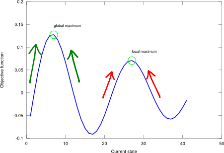
Note that the heuristic operates at the node level (not at the path level like a step cost). It’s a state fitness function and it doesn’t add-up over the traversal of nodes. With a good heuristic function, the complexity of the search procedure can be reduced substantially. The amount of the reduction, though, depends on the particular problem at hand and on the quality of the heuristic. And there is no free lunch here: developing a bespoke solution for a specific problem entails carefully designing a tailored heuristic, which generally works well only for this particular scenario.

A good heuristic never overestimates the number of steps to the solution. This requirement is commonly known as “admissibility”. In order to comply with it, the heuristic usually represents the cost of an optimal solution to a relaxed problem, which is the original problem without some constraints. Additionally, a heuristic may also show “consistency” if its estimated cost is monotonically non-increasing as it approaches the goal state (this is a stronger condition). As a rule of thumb, it is generally better to use a heuristic function with higher values provided it is consistent and that its computation is short.

Greedy search in detail

Greedy search (GS) is an informed search method that tries to expand the node that is strictly closest to the goal, assuming that it is likely to lead to a solution quickly. Thus, it evaluates neighbouring nodes by using only the heuristic function. Note that GS is not optimal nor complete (the immediate short-term benefit may not be the optimum one in the long run), but it is often efficient. Regarding its implementation, the former BES procedure is used with an anonymous evaluation function that returns the heuristic alone , see Figure 2.

Figure 2. Greedy search algorithm.

## @deftypefn {Function File} {@var{solution} =} greedy_search (@var{problem}, @var{start}, @var{finish}, @var{treegraph}, @var{heuristic})
## Greedy search algorithm.
##
## PRE:
## @var{problem} must be the cost-weighted adjacency matrix.
## @var{start} must be the starting node index.
## @var{finish} must be the finishing node index.
## @var{treegraph} must be the tree/graph version flag. 0 is tree-version.
## @var{heuristic} must be the heuristic vector.
##
## POST:
## @var{solution} is the solution path. State set to zero if failure.
## @end deftypefn

## Author: Alexandre Trilla <alex@atrilla.net>

function [solution] = greedy_search(problem, start, finish, treegraph,
  heuristic)

  % eval func is anonymous and returns heuristic
  solution = best_first_search(problem, start, finish, treegraph, ...
    @(cost) cost(2), heuristic);

endfunction

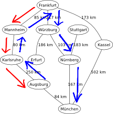
Following the UCS example with the graphical map of Germany, the heuristic of use for GS is based on the distance to München by motorways provided by ViaMichelin (a close resemblance to a straight-line distance). The resulting path from Frankfurt to München is the same, via Wurzburg and Nurnberg. However, GS resolves the problem in 6.96ms, while UCS does it in 12.4ms (almost double the time). Indeed, GS is more effective than UCS finding the best path in this informed environment.

The iterative deepening search algorithm

Iterative deepening search (IDS) combines the benefits of breadth-first and depth-first search: it has modest memory requirements (linear space complexity), and it is complete and optimal when the branching factor is finite, with a time complexity comparable to breadth-first ( is the depth of the solution). IDS works in tandem with depth-limited search and finds the best depth limit with a gradually increasing loop, see Figure 1. In general, IDS is the preferred uninformed search method when the search space is large and the depth of the solution is not known.

Figure 1. Iterative deepening search algorithm.

## @deftypefn {Function File} {@var{solution} =} iterative_deepening_search(@var{problem}, @var{start}, @var{finish})
## Iterative deepening search algorithm.
##
## PRE:
## @var{problem} must be the cost-weighted adjacency matrix.
## @var{start} must be the starting node index.
## @var{finish} must be the finishing node index.
##
## POST:
## @var{solution} is the solution path. State set to zero if there
## is no solution.
## @end deftypefn

## Author: Alexandre Trilla <alex@atrilla.net>

function [solution] = iterative_deepening_search(problem, start, ...
  finish)

  limit = 1;
  while (limit)
    solution = depth_limited_search(problem, start, finish, limit);
    limit += 1;
    if (solution.state ~= 1)
      break;
    endif
  endwhile

endfunction

With IDS you have got to the end of the section that deals with uninformed search strategies. What follows is the journey through informed search methods, where environment knowledge is incorporated in the search procedure in order to guide it (and thus make it more effective). Stay tuned!