Uniform-cost search (UCS) is somewhat similar to breadth-first search (BFS), but this new approach seeks the minimum-cost path instead of the shallowest path. This is accomplished by using a priority queue (ordered by path cost) for the frontier, and an extra check in case a shorter path to a frontier state is discovered while traversing the graph, see Figure 1.

Figure 1. Uniform-cost search algorithm.

## @var{problem} must be the cost-weighted adjacency matrix.
## @var{start} must be the starting node index.
## @var{finish} must be the finishing node index.
## @var{treegraph} must be the tree/graph version flag. 0 is tree-version.
##
## POST:
## @var{solution} is the solution path. State set to zero if failure.
## @end deftypefn

## Author: Alexandre Trilla <alex@atrilla.net>

function [solution] = uniform_cost_search(problem, start, ...
  finish, treegraph)

  % inits
  node.state = start;
  node.parent = [];
  node.cost = 0;
  
  if (node.state == finish)
    solution = node;
  else
    frontier = [node];
    explored = [];
    found = 0;
    while (~found)
      if (numel(frontier) == 0)
        solution.state = 0;
        found = 1;
        break;
      endif
      % pop frontier, lowest cost node
      testNode = frontier(1);
      testIdx = 1;
      for i = 2:numel(frontier)
        if (frontier(i).cost < testNode.cost)
          testNode = frontier(i);
          testIdx = i;
          continue;
        endif
      endfor
      frontier = ...
        frontier([1:(testIdx-1) (testIdx+1):numel(frontier)]);
      node = testNode;
      % check
      if (node.state == finish)
        solution = node;
        break;
      endif
      % explore
      if (treegraph)
        explored(numel(explored)+1) = node.state;
      endif
      for i = 1:size(problem, 2)
        if (problem(node.state, i)>0)
          if (i ~= node.state)
            child.state = i;
            path = node.parent;
            path = [path node.state];
            child.parent = path;
            child.cost = node.cost + problem(node.state, i);
            notExpl = 1;
            if (treegraph)
              notExpl = ~sum(explored == i);
            endif
            if (notExpl)
              inFront = 0;
              for j = 1:numel(frontier)
                if (frontier(j).state == i)
                  inFront = 1;
                  if (frontier(j).cost > child.cost)
                    frontier(j) = child;
                  endif
                  break;
                endif
              endfor
              if (~inFront)
                frontier = [frontier child];
              endif
            endif
          endif
        endif
      endfor
    endwhile
  endif

endfunction

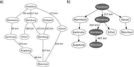
UCS is complete and optimal in general. Borrowing the same example from the Wikipedia, the shortest path (wrt distance) from Frankfurt to Münich is via Wüzburg and Nürnberg, which adds up to 487km (not 675km like the solution found via Kassel with BFS), see Figure 2.

Figure 2. UCS applied on the graphical map of Germany. Source: Wikipedia. a) Problem description. b) Search tree.

Regarding its algorithmic complexity, UCS depends on path costs rather than on depths, so it is not easily characterised in terms of branching factor and depth of the solution (when all step costs are the same, UCS and BFS are pretty similar, i.e., they both have similar exponential complexities). However, since UCS is expected to explore all the nodes at the goal’s depth, it will usually do more work unnecessarily. In the following posts you’ll see how the completeness and optimality features can be relaxed to favour the algorithmic complexity of a search procedure. Stay up to date!