The same principles that reign in local search methods for discrete spaces also apply to continuous spaces, i.e., start at some random place and take little steps toward the maximum. Taking into account that most real-world problems are continuous, it is no surprise that the literature on this topic is vast. For conventional, well-understood problems, a gradient-based technique may be the best approach you can take. It’s really worth it having a look at how they work!
Search objectives in continuous spaces are broadly described by real-valued smooth functions , i.e., twice differentiable functions. Then, the gradient/derivative of this objective function is a vector that gives the magnitude and direction of the steepest slope:
With this you can perform steepest-ascent hill climbing by updating the current state (initially random) according to the formula:
where is a small constant often called the “step size”, which determines the amount of contribution that the gradient has in the update process. Little by little, one step at a time, the algorithm will get to the maximum. However, having to calculate the gradient expression analytically by hand is a pain in the arse. Instead, you can compute an empirical gradient (i.e., numerically) by evaluating the response to small increments in each dimension/variable.
In order to see the gradient ascent algorithm in action, I will use a parallel LC resonant band-pass filter, see Figure 1.
Figure 1. Parallel LC resonant band-pass filter. Source: All About Circuits.
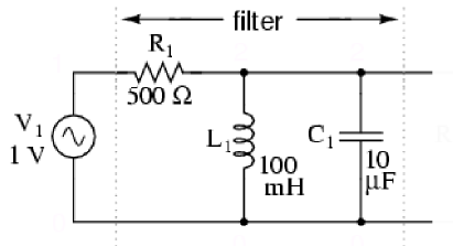
The goal here is to find the band-pass frequency (a real number) of this filter. Recall that this is to be done numerically (the resonance of this circuit is well known to be , so at 159.15Hz for these component values: L=100mH, C=10uF). Thus, the magnitude of the transfer function of this filter is given as follows:
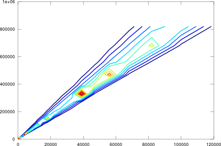
Note that is the magnitude of the impedance of the parallel LC circuit. The landscape plot of this function (that is the frequency domain) is shown in Figure 2. Note that this particular problem is somewhat tricky for gradient ascent, because the derivative increases as it approaches the maximum, so it may easily diverge during the update process (a really small step size is mandatory here). Other objective (convex) functions like the exponential error are expected to be more suitable because they are normally smoother around the extrema.
Figure 2. Gradient ascent applied on the magnitude function of a parallel LC resonant band-pass filter.

Despite the high peakedness of the he objective function, the gradient ascent method is able to find the maximum in a breeze. The complete code listing is shown in Figure 3. Regarding its computational complexity, the space is bounded by the size of the variables vector, but the time depends on the specific shape of the landscape, the size of the step, etc.
Figure 3. Gradient ascent algorithm.
-- Gradient ascent algorithm.
--
-- PRE:
-- objfun - objective funciton to maximise (funciton).
-- var - variables, starting point vector (table).
-- step - step size (number).
--
-- POST:
-- Updates var with the max of objfun.
--
-- Loop while evaluation increases.

function gradient_ascent(objfun, var, step)
  local epsilon = 1e-4
  local feval = objfun(var)
  local grad = {}
  for i = 1, #var do
    table.insert(grad, 0)
  end
  local newvar = {}
  for i = 1, #var do
    table.insert(newvar, 0)
  end
  while (true) do
    local preveval = feval
    -- calc grad
    for i = 1, #var do
      local value = var[i]
      var[i] = value + epsilon
      local right = objfun(var)
      var[i] = value - epsilon
      local left = objfun(var)
      var[i] = value
      grad[i] = (right - left) / (2 * epsilon)
    end
    -- new var
    for i = 1, #var do
      newvar[i] = var[i] + step * grad[i]
    end
    -- eval
    feval = objfun(newvar)
    if (feval > preveval) then
      -- update var
      for i = 1, #var do
        var[i] = newvar[i]
      end
    else
      break
    end
  end
end
You must note, though, that this is a simple optimisation technique that works well if one single global extremum is present, but that more refined tweaks need to be applied if the objective function gets more complex. In the end, gradient ascent is complete but non-optimal. A typical and effective way to add robustness and speed up the process is to take as a time-dependent function (measured by the number of iterations in the loop) that settles the learning capability, pretty much like the simulated annealing algorithm. Other strategies take into account the momentum of the learning process in order to speed it up at times, in addition to avoiding local maxima. There is also the venerable Newton-Raphson algorithm, which makes use of the Hessian matrix (involving second derivatives) to optimise the learning path, although it can be somewhat tedious to run because it involves matrix inversion. This is all a rich and endless source of PhD topics.
Having a basic knowledge of such gradient-based methods, though, opens up a full range of possibilities, such as the use of Artificial Neural Networks (ANN). ANN’s are very fashion nowadays because of the disruption of deep learning. I know I’m being a little ahead of time with this technique, but it’s just so appealing to tackle so many problems that I can’t resist (note that an ANN is part of the A.I. Maker logo). In the next post, you’ll see how ANN’s can be easily learnt and deployed by directly applying gradient-based methods on complex functions. Stay tuned!