The depth-limited search algorithm

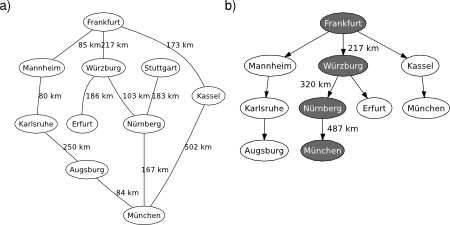
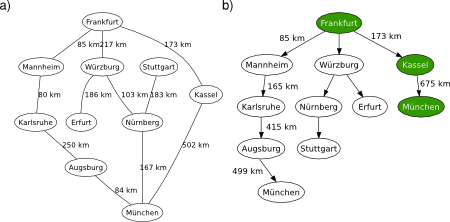
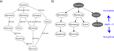
The depth-limited search (DLS) method is almost equal to depth-first search (DFS), but DLS solves the infinite state space problem because it bounds the depth of the search tree with a predetermined limit . Nodes at this depth limit are treated as if they had no successors. Thus, its time complexity is and its space complexity is ( is the branching factor). Note that DPS can be viewed as a special case of DLS with an infinite limit (in a sense, DLS is a more general approach). Also note that DLS is still incomplete (the given limit may be less than the depth of the solution) and nonoptimal (it may be greater), see Figure 1. However, in order to have an informed upper bound of the optimal depth limit, you can reasonably use the diameter of the state space (i.e., the longest shortest path between any two nodes defined by the problem).

Figure 1. DLS applied on the graphical map of Germany. Depth of solution from Frankfurt to München is 2. Source: Wikipedia. a) Problem description. b) Search tree.

DLS applied on the graphical map of Germany.
DLS applied on the graphical map of Germany

The tree search version of DLS can be conveniently implemented by exploiting recursivity, see Figure 2. The frontier is not explicitly declared but inherently maintained in the stack of calls.

Figure 2a. Depth-limited tree search algorithm.

## @deftypefn {Function File} {@var{solution} =} depth_limited_search (@var{problem}, @var{start}, @var{finish}, @var{limit})
## Recursive implementation of depth-limited tree search.
##
## PRE:
## @var{problem} must be the cost-weighted adjacency matrix.
## @var{start} must be the starting node index.
## @var{finish} must be the finishing node index.
## @var{limit} must be the depth limit.
##
## POST:
## @var{solution} is the solution path. Zero if standard failure
## (no solution). One if cutoff failure (no solution within the
## depth limit).
## @end deftypefn

## Author: Alexandre Trilla <alex@atrilla.net>

function [solution] = depth_limited_search(problem, start, ...
  finish, limit)

  node.state = start;
  node.parent = [];
  node.cost = 0;
  solution = recursive_dls(node, problem, finish, limit);

endfunction

Figure 2b. Recursive implementation of depth-limited tree search.

## @deftypefn {Function File} {@var{solution} =} recursive_dls(@var{node}, @var{problem}, @var{finish}, @var{limit})
## Recursive implementation of depth-limited tree search.
##
## PRE:
## @var{node} must be the starting node.
## @var{problem} must be the cost-weighted adjacency matrix.
## @var{finish} must be the finishing node index.
## @var{limit} must be the depth limit.
##
## POST:
## @var{solution} is the solution path. State set to zero if standard
## failure (no solution). One if cutoff failure (no solution within
## the depth limit).
## @end deftypefn

## Author: Alexandre Trilla <alex@atrilla.net>

function [solution] = recursive_dls(node, problem, finish, limit)

  if (node.state == finish)
    solution = node;
  elseif (limit == 0)
    solution.state = 1;
  else
    cutoff = 0;
    for i = 1:size(problem, 2)
      if (problem(node.state, i)>0)
        if (i ~= node.state)
          % expand search space
          child.state = i;
          path = node.parent;
          path = [path node.state];
          child.parent = path;
          child.cost = node.cost + problem(node.state, i);
          result = recursive_dls(child, problem, finish, ...
            limit - 1);
          if (result.state == 1)
            cutoff = 1;
          elseif (result.state ~= 0)
            solution = result;
            return;
          endif
        endif
      endif
    endfor
    if (cutoff)
      solution.state = 1;
    else
      solution.state = 0;
    endif
  endif

endfunction

Notice that DLS can terminate with two kinds of failure: the “no solution” standard failure, and the “cutoff” failure that indicates no solution within the given depth limit. In the next post, you are going to see how the accurate tracking of the given depth limit enables a DLS-inspired algorithm to be both complete and optimal. Stay tuned!

Depth-first search

Depth-first search (DFS) is a strategy that expands the deepest node in the current frontier. Thus, the frontier is based on a Last-In First-Out node container. The DFS approach is not optimal nor complete. The solution it yields is not based on any particular cost criterion: depending on which path is explored first the result may vary. Let’s say it is a somewhat “daring” approach because it takes the first path it comes across and goes to the end with it hoping it leads to the destination as soon as possible. This gives DFS a space complexity advantage over its breadth-first counterpart. While DFS has an equally concerning exponential time complexity , where is the branching factor and is the maximum depth of the search tree, it has a linear space complexity , which makes it more appealing for an effective (and feasible) implementation. DFS saves a lot of memory because it needs to store only one path from the root of the search tree to a leaf node.

In order to implement the DFS algorithm, let’s now reap the benefit of having coded the abstract data type (ADT) search procedure. Note that DFS can be easily specified if the ADT-search algorithm is given a handle to a function that manages the frontier as a stack, see Figure 1.

Figure 1. Stack insertion function.

## @deftypefn {Function File} {@var{insertion} =} ins_fifo(@var{frontier}, @var{node})
## Stack insertion.
##
## PRE:
## @var{frontier} must be a struct array for the frontier.
## @var{node} must be a struct for the node.
##
## POST:
## @var{insertion} is the extended frontier.
## @end deftypefn

## Author: Alexandre Trilla <alex@atrilla.net>

function [insertion] = ins_lifo(frontier, node)

  insertion = [node frontier];

endfunction

Are you wondering why all these search strategies have such a similar implementation pattern? Does all seem to be a matter of tweaking a line or two and giving it a new name? You are right. They don’t need to be so similar. In the following post you’ll see how DFS is implemented applying recursivity, for development convenience, and how its complexity features can also be bounded. Stay tuned!

Uniform-cost search

Uniform-cost search (UCS) is somewhat similar to breadth-first search (BFS), but this new approach seeks the minimum-cost path instead of the shallowest path. This is accomplished by using a priority queue (ordered by path cost) for the frontier, and an extra check in case a shorter path to a frontier state is discovered while traversing the graph, see Figure 1.

Figure 1. Uniform-cost search algorithm.

## @var{problem} must be the cost-weighted adjacency matrix.
## @var{start} must be the starting node index.
## @var{finish} must be the finishing node index.
## @var{treegraph} must be the tree/graph version flag. 0 is tree-version.
##
## POST:
## @var{solution} is the solution path. State set to zero if failure.
## @end deftypefn

## Author: Alexandre Trilla <alex@atrilla.net>

function [solution] = uniform_cost_search(problem, start, ...
  finish, treegraph)

  % inits
  node.state = start;
  node.parent = [];
  node.cost = 0;
  
  if (node.state == finish)
    solution = node;
  else
    frontier = [node];
    explored = [];
    found = 0;
    while (~found)
      if (numel(frontier) == 0)
        solution.state = 0;
        found = 1;
        break;
      endif
      % pop frontier, lowest cost node
      testNode = frontier(1);
      testIdx = 1;
      for i = 2:numel(frontier)
        if (frontier(i).cost < testNode.cost)
          testNode = frontier(i);
          testIdx = i;
          continue;
        endif
      endfor
      frontier = ...
        frontier([1:(testIdx-1) (testIdx+1):numel(frontier)]);
      node = testNode;
      % check
      if (node.state == finish)
        solution = node;
        break;
      endif
      % explore
      if (treegraph)
        explored(numel(explored)+1) = node.state;
      endif
      for i = 1:size(problem, 2)
        if (problem(node.state, i)>0)
          if (i ~= node.state)
            child.state = i;
            path = node.parent;
            path = [path node.state];
            child.parent = path;
            child.cost = node.cost + problem(node.state, i);
            notExpl = 1;
            if (treegraph)
              notExpl = ~sum(explored == i);
            endif
            if (notExpl)
              inFront = 0;
              for j = 1:numel(frontier)
                if (frontier(j).state == i)
                  inFront = 1;
                  if (frontier(j).cost > child.cost)
                    frontier(j) = child;
                  endif
                  break;
                endif
              endfor
              if (~inFront)
                frontier = [frontier child];
              endif
            endif
          endif
        endif
      endfor
    endwhile
  endif

endfunction

UCS is complete and optimal in general. Borrowing the same example from the Wikipedia, the shortest path (wrt distance) from Frankfurt to Münich is via Wüzburg and Nürnberg, which adds up to 487km (not 675km like the solution found via Kassel with BFS), see Figure 2.

Figure 2. UCS applied on the graphical map of Germany. Source: Wikipedia. a) Problem description. b) Search tree.

UCS applied on the graphical map of Germany.
UCS applied on the graphical map of Germany

Regarding its algorithmic complexity, UCS depends on path costs rather than on depths, so it is not easily characterised in terms of branching factor and depth of the solution (when all step costs are the same, UCS and BFS are pretty similar, i.e., they both have similar exponential complexities). However, since UCS is expected to explore all the nodes at the goal’s depth, it will usually do more work unnecessarily. In the following posts you’ll see how the completeness and optimality features can be relaxed to favour the algorithmic complexity of a search procedure. Stay up to date!

Refactoring breadth-first search

For the sake of generality, I have refactored the code of the breadth-first search (BFS) algorithm in order to accommodate both the tree and the graph-search versions. This has to do with the ability of the algorithm to deal with redundant paths, whether if they are to be taken into account (graph-search, as it is described in pseudocode in the book) or not (tree-search). The bulk of the code has been redefined as a generic abstract data type (ADT) search algorithm, which has an additional flag to use the explored set or not, see Figure 1 (changes are highlighted).

Figure 1. Abstract data type search algorithm.

## @deftypefn {Function File} {@var{solution} =} adt_search (@var{problem}, @var{start}, @var{finish}, @var{treegraph}, @var{insert})
## Abstract data type search algorithm.
##
## PRE:
## @var{problem} must be the cost-weighted adjacency matrix.
## @var{start} must be the starting node index.
## @var{finish} must be the finishing node index.
## @var{treegraph} must be the tree/graph version flag. Zero is
## tree-version.
## @var{insert} must be function handle to manage the insertion into
## the frontier.
##
## POST:
## @var{solution} is the solution path. State set to zero if failure.
## @end deftypefn

## Author: Alexandre Trilla <alex@atrilla.net>

function [solution] = adt_search(problem, start, ...
  finish, treegraph, insert)

  % inits
  node.state = start;
  node.parent = [];
  node.cost = 0;

  if (node.state == finish)
    solution = node;
  else
    frontier = [node];
    explored = [];
    found = 0;
    while (~found)
      if (numel(frontier) == 0)
        solution.state = 0;
        found = 1;
        break;
      endif
      % pop frontier
      node = frontier(1);
      frontier = frontier(2:end);
      % explore
      if (treegraph)
        explored(numel(explored)+1) = node.state;
      endif
      for i = 1:size(problem, 2)
        if (problem(node.state, i)>0)
          if (i ~= node.state)
            % by default, continue exploration
            notExpl = 1;
            if (treegraph)
              notExpl = ~sum(explored == i);
            endif
            if (notExpl)
              inFront = 0;
              for j = 1:numel(frontier)
                if (frontier(j).state == i)
                  inFront = 1;
                  break;
                endif
              endfor
              if (~inFront)
                % expand search space
                child.state = i;
                path = node.parent;
                path = [path node.state];
                child.parent = path;
                child.cost = node.cost + problem(node.state, i);
                % check goal
                if (i == finish)
                  solution = child;
                  found = 1;
                  break;
                else
                  frontier = insert(frontier,child);
                endif
              endif
            endif
          endif
        endif
      endfor
    endwhile
  endif

endfunction

Note that the ADT-search algorithm is also given a function handle to manage the insertion of a node into the frontier. The rationale for doing it is mainly to avoid the Don’t-Repeat-Yourself principle, i.e., the pragmatic programmer’s tip number 11. The benefit of this will come when we get to depth-first search. Stay tuned! Now, if this ADT-search algorithm is given a handle to a function that manages the frontier as a queue, see Figure 2, the functional behaviour of BFS remains the same.

Figure 2. Queue insertion function.

## @deftypefn {Function File} {@var{insertion} =} ins_fifo(@var{frontier}, @var{node})
## Queue insertion.
##
## PRE:
## @var{frontier} must be a struct array for the frontier.
## @var{node} must be a struct for the node.
##
## POST:
## @var{insertion} is the extended frontier.
## @end deftypefn

## Author: Alexandre Trilla <alex@atrilla.net>

function [insertion] = ins_fifo(frontier, node)

  insertion = [frontier node];

endfunction

A final note on the application scenario of BFS

The BFS algorithm (and in fact the rest of search routines you will see shortly) is to be deployed on environments that are deterministic, observable, static, and completely known. Otherwise, if the application scenario at hand does not display these characteristics, you simply can’t design an agent that performs actions to accomplish its goals with BFS.
BFS is a search strategy that seeks the shallowest path to the solution, it is complete (so it always finds a solution if there is one, at least), it is optimal for unit step costs, but it has exponential space complexity, which makes it infeasible for large-space search problems. Also note that the description of the search problem must be discrete, therefore the trees, graphs and their adjacency matrices. If continuous environments are to be searched with these methods, they must be discretised first, thus yielding a quantisation error according to the granularity of the grid of use. Or else use some common sense to reasonably represent the problem in discrete and tractable terms, like the BFS example with the map of Germany.

Breadth-first search

The first topic that is tackled in the AIMA book is problem solving by searching over a graphical structure. The overall operation of this family of algorithms is based on traversing the given graph, keeping unexplored nodes in a container called the “frontier”, and then exploring these nodes, one at a time. The strategy to conduct the search process, thus, depends on how nodes are managed with the frontier. If the frontier is treated as a queue, i.e., First-In First-Out, then the graph traversal is progressed via a breadth-first criterion, whereas if the frontier is used as a stack, i.e., Last-In First-Out, then the search algorithm expands by depth-first.

There is another issue regarding the redundancy of the paths. If the search algorithm does not take into account which nodes it explores along the way, it may traverse them more than once. This is called a tree-search algorithm. Instead, if it makes sure to not traverse the same node twice, it is called a graph-search algorithm. The suitability of one or the other depends on the nature of the objective problem at hand (and the ability of the searcher to trace its own footsteps in case it reaches a dead end).

Also, some search algorithms operate with the support of some guiding knowledge (that is like a kind of compass that points to the right direction), which are called informed search strategies, while others go around blindly without any knowledge at all about what next action is best, which are called uninformed search strategies. What must be common to all problem definitions, though, is that the step costs from one node to another be non-negative.

Based on the former premises, several search routines are typically defined. What follows are the details of the breadth-first search (BFS) algorithm.

BFS in detail

Breadth-first is an uninformed search strategy that seeks the shallowest path to the solution. Since it uses a FIFO queue for the frontier, the nodes at a given depth are always expanded before any nodes at the next level. This algorithm is commonly implemented following a graph-search template, see Figure 1, also available on the GitHub repository.

Figure 1. Breadth-first search algorithm.

## @deftypefn {Function File} {@var{solution} =} breadth_first_search (@var{problem}, @var{start}, @var{finish})
## Breadth-first search on a graph.
##
## PRE:
## @var{problem} must be the cost-weighted adjacency matrix.
## @var{start} must be the starting node index.
## @var{finish} must be the finishing node index.
##
## POST:
## @var{solution} is the solution path. State set to zero if failure.
## @end deftypefn

## Author: Alexandre Trilla <alex@atrilla.net>

function [solution] = breadth_first_search(problem, start, finish)

% inits
node.state = start;
node.parent = [];
node.cost = 0;

if (node.state == finish)
    solution = node;
else
    frontier = [node];
    explored = [];
    found = 0;
    while (~found)
        if (numel(frontier) == 0)
            solution.state = 0;
            found = 1;
            break;
        endif
        % pop frontier
        node = frontier(1);
        frontier = frontier(2:end);
        % explore
        explored(numel(explored)+1) = node.state;
        for i = 1:size(problem, 2)
            if (problem(node.state, i)>0)
                if (i ~= node.state)
                    if (~sum(explored == i))
                        inFront = 0;
                        for j = 1:numel(frontier)
                            if (frontier(j).state == i)
                                inFront = 1;
                                break;
                            endif
                        endfor
                        if (~inFront)
                            % expand search space
                            child.state = i;
                            path = node.parent;
                            path = [path node.state];
                            child.parent = path;
                            child.cost = node.cost + ...
                                problem(node.state, i);
                            % check goal
                            if (i == finish)
                                solution = child;
                                found = 1;
                                break;
                            else
                                frontier = [frontier child];
                            endif
                        endif
                    endif
                endif
            endif
        endfor
    endwhile
endif

endfunction

The gist of the BFS approach is to explore all possible options at a given point/level before making a decision on what to do next (i.e., the following node to be explored). Thus, it’s kind of hesitant. This has important implications on the computational complexity of this algorithm. Both time and space complexities are exponential with respect to the branching factor , i.e., the number of nodes that the search tree generates at a given level, and the depth of the solution: . Therefore, memory requirements are a bigger problem for BFS than is the execution time. In general, exponential-complexity search problems cannot be solved by uninformed methods for any but the smallest instances.

As a practical example, let’s use the graphical map of Germany from Wikipedia, see Figure 2a. If you apply BFS from Frankfurt to München, for example, the algorithm resolves the problem via Kassel, which is the shallowest path (two hops), see Figure 2b. This is fine. However, this is by no means the least costly solution as the distance amounts to 675km: it is not optimum in this distance-cost sense.

Figure 2. BFS applied on the graphical map of Germany. Source: Wikipedia. a) Problem description. b) Search tree.

BFS applied on the graphical map of Germany.
BFS applied on the graphical map of Germany

BFS may be somewhat misleading in this case because it treats physical dimensions as if they all weighed the same. But there is room for improvement here. So stay tuned for the next post. There you will deal with the optimum search strategy that accounts for the lowest-cost path to resolve the traversal of the graph.