A closer look at problem state encoding in genetic algorithms through electronics

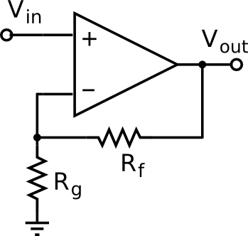
Encoding problem state information in a genetic algorithm (GA) is one of the most cumbersome aspects of its deployment. GA deals with binary vectors, so this is the format that you must comply to in order to find optimum solutions with this technique. And depending on which strategy you choose to do it, the solution of the search process may be different, and/or the GA algorithm may take more or less time (and/or space) to reach it. In order to display some of these issues, I will go through a complete example with an electronic circuit in this post. Specifically, the circuit under analysis will be a non-inverting amplifier built with an OP07 operational amplifier, see Figure 1. The goal of this discrete optimisation problem will be to find the optimum values of its two resistors Rf and Rg (over a finite set, so that they may be available in the store and the circuit be implementable) that maximise the symmetric excursion of a 1V peak input sinusoidal signal without clipping. Let’s synthesise this circuit with GA!

Figure 1. Schematic of a non-inverting amplifier. Source: Wikipedia.

Schematic of a non-inverting amplifier
Schematic of a non-inverting amplifier.

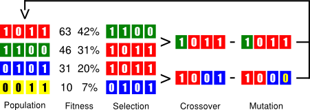
First step: encode each resistor value alone into a binary array. It is a good approach to represent the bits of an integer number, where the weight of each bit is directly related to a specific weight of the resistive spectrum, i.e., the most significant bits always correspond to high resistor values (and vice-versa), see Figure 2. I had also tried to follow the colour-based encoding that resistors display, i.e., like a mantissa and an exponent, but it’s been much of a failure, which I suspect is given by the non-linear relation between bit weight and resistance value. Note that you must still check that the represented number is within the accepted range of resistor values. Otherwise, discard it by assigning a bad fitness score so that it is likely to disappear during the evolution process. In this example, I’ll be using the 10% standard resistor values, from 10 ohm to 820k ohm (so, 60 different values in total, 6 bits).

Figure 2. Resistor value encoding and crossover.

Resistor value encoding and crossover
Resistor value encoding and crossover.

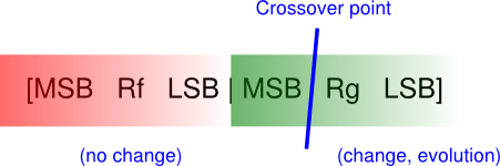
Next, encode the two resistor values in an array to create an initial population. To this end, append one resistor to the other to build an aggregate individual, like [Rf Rg], again see Figure 2. When having to combine them, the crossover point will keep the value of one resistor stable while evolving the other under improvement, which makes perfect sense.

Now, the output function of the non-inverting amplifier is given by:

and the fitness function used to evaluate the effectiveness of a solution is mainly driven by the inverse of the error of the symmetric excursion of (recall that greater scores are for better individuals):

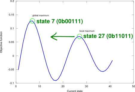
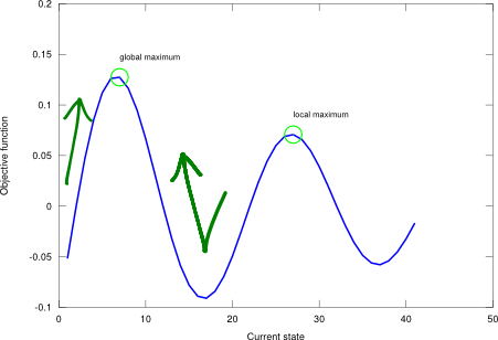
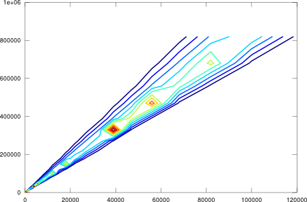
Taking into account that with a power supply of 15V the OP07 saturates at about 12V, let’s fix the maximum symmetric excursion of the output to 20V (i.e., ) to avoid signal clipping. Having all that set, you’re ready to start optimising. Having a look at the fitness surface that the GA algorithm will deal with, see Figure 3, it shows that it will have a hard time dealing with so many extrema. Note that all maxima are located on a 9x slope line, which indicates that the solution must maintain a ratio of 9 between Rf and Rg. Also note that resistors placed on the lower end of the resistance range tend to be more stable and consume more power, while the ones placed on the higher end of the range draw less current but are more unstable. Since none of these considerations are included in the fitness function, the GA procedure may end on any of these local maxima, e.g, and , with a fitness score of .

Figure 3. Fitness surface plot.

Fitness surface plot
Fitness surface plot.

The performance of a brute-force exhaustive iterative search solution is taken for reference here, which has a computational complexity in time of , where is amount of possible resistor values (i.e., 60), and is the number of resistors in circuit (i.e., 2). This yields a search space of 3600 states. No matter how fancy GA’s may be, for such small search space, exhaustive linear search is much faster (it takes less than a second, while GA takes 5 secs). With 4 resistors, though, the search space is over 12M and the two approaches take about 10 secs. Over this bound, GA is able to perform better. Long are the days when engineers had to assemble the prototype circuits on a breadboard to optimise the numerical values of each of the components, see this video at 6:15.

The genetic algorithms

A genetic algorithm (GA) is a variant of stochastic beam search, which involves several search points/states concurrently (similar to the shotgun approach noted in the former post), and somehow combines their features according to their performance to generate better successor states. Thus, GA differs from former approaches like simulated annealing that only rely on the modification and evolution of a single state.

In GA, each search state, aka individual, encodes the problem information, usually as a binary array. GA begins with a set of randomly generated states, called the population. Then, it iterates over the chain of evolution for a determined number of rounds, see Figure 1, described as follows:

  1. Fitness evaluation: each state is scored wrt some effectiveness criterion (higher values for better states).
  2. Selection: states are randomly sampled with a specific probability according to their fitness value.
  3. Crossover: selected individuals are randomly shuffled or combined at a specific point.
  4. Mutation: child individuals may flip some of their bits (each one with independent probability).

Figure 1. Chain of evolution in genetic algorithms.

Chain of evolution in genetic algorithms
Chain of evolution in genetic algorithms.

The advantage with GA comes from the ability of crossover to combine large blocks of bits (i.e., state information) that have evolved independently to perform a specific useful function. However, the successful use and application of GA requires careful engineering of the state representation and its encoding (in addition to the more common optimisation parameters like the population size or the number of evolution rounds). This has a deep impact on the performance of the algorithm. Figure 2 shows an example objective landscape where the state-space number is represented as a binary array of 5 bits (unsigned integer).

Figure 2. Genetic algorithm applied on a one-dimensional state-space landscape described by an example objective function .

Genetic algorithm on a state-space landscape
Genetic algorithm on a state-space landscape.

GA belongs to a family of metaheuristics, which are algorithms designed to tackle ill-defined functions where a clear and definite objective is impossible to use. GA are adequate for black box search processes. Figure 3 implements the GA algorithm. Note how no explicit objective function is given. Instead, an initial population and a fitness function are passed to begin the search for the optimum.

Figure 3. Genetic algorithm.

-- Genetic algorithm.
--
-- PRE:
-- population - set of individuals (table).
-- fitness - evaluate individual (function).
--
-- POST:
-- solution - solution state (table).
--
-- Each individual (state) is a binary array.
-- Population is ordered from best to worst according to fitness. It
-- must be greater than one.
-- Fitness is normalised from 0 (bad) to 1 (good).

local function sort_population(population, fitness)
  local function comp(x, y)
    return (fitness(x) < fitness(y))
  end
  return table.sort(population, comp)
end

local function random_selection(population, fitness)
  local fit = {}
  local sumfit = 0
  for i = 1, #population do
    local fitIndi = fitness(population[i])
    table.insert(fit, fitIndi)
    sumfit = sumfit + fitIndi
  end
  fit[1] = fit[1] / sumfit
  for i = 2, #fit do
    fit[i] = fit[i] / sumfit + fit[i-1]
  end
  local x, y
  local rx = math.random()
  local ry = math.random()
  for i = 1, #fit do
    if (rx < fit[i]) then
      x = population[i]
      break
    end
  end
  for i = 1, #fit do
    if (ry < fit[i]) then
      y = population[i]
      break
    end
  end
  return x, y
end

local function reproduce(x, y)
  local point = math.floor(math.random() * #x) + 1
  local child = {}
  for i = 1, point do
    child[i] = x[i]
  end
  for i = point + 1, #x do
    child[i] = y[i]
  end
  return child
end

local function mutate(x)
  for i = 1, #x do
    if (math.random() < 0.1) then
      x[i] = math.abs(x[i] - 1)
    end
  end
end

function genetic_algorithm(population, fitness)
  local solution
  for epoch = 1, 100 do
    sort_population(population, fitness)
    local new_population = {}
    for i = 1, #population do
      local x, y = random_selection(population, fitness)
      local child = reproduce(x, y)
      if (math.random() < 0.05) then
        mutate(child)
      end
      table.insert(new_population, child)
    end
    population = new_population
  end
  return population[1]
end

The GA algorithm suggested in AIMA does not posit any similarity with real world reproductive systems, though. Is it reasonable to prevent inbreeding? In nature, close genetic relation results in disorders. Such issues are not discussed, but they don’t seem to have much of an impact for function optimisation purposes (in this particular case, mutation may add value here by creating a new individual).

Finally, regarding the computational complexities of GA, the space complexity is given by the number of individuals in the population , and the time complexity is given by the intermediate processes of the evolution chain. I guess one the critical points is ranking the individuals according to their fitness value for sampling. In the former implementation, Lua’s table.sort function (based on quicksort) is used. However, I would expect an overall for a tractable amount of instances. Depending on how fine you are with respect to your specific problem, several options may fit. Use your most sensible and plausible bound here (and test it!).

The simulated annealing algorithm

Simulated annealing (SA) is a local search method that combines the features of hill climbing (incomplete, effective) with the features of a random walk (complete, ineffective) in a way that yields both efficiency and completeness. The overall working principle is quite similar to hill climbing (to move upwards to the maximum), but now the short-term decisions of where to go next are stochastic. If a random choice improves the situation, it is always accepted. Otherwise, the SA algorithm accepts the “bad” move with a given transition probability. This probability decreases exponentially with the badness of the move, and a temperature factor, which allows doing such irrational moves only during a short period of time (recall that the transition is to a worse state). Empirically, though, it can be shown that under certain circumstances (i.e., with tailored parameters), this may favour leaving a local maximum for heading toward the optimum, see Figure 1. The probability associated to this turning action is called the Boltzmann factor, and quantifies the likelihood that a system transitions to a new energy state at a given temperature.

Figure 1. Simulated annealing applied on a one-dimensional state-space landscape described by an example objective function .

Simulated annealing on a state-space landscape
Simulated annealing on a state-space landscape.

The origin of the SA algorithm is found in the metallurgic tempering process, where high temperature is first applied to a metal to produce an atomic disorder, and then it is cooled down gradually in order to align the atoms and leave the system in a crystalline state. The analogy with the local search problem is that SA first allows lots of possibilities (high temperature) hoping to cover the optimum with greater chance, and then the system is brought to a stable state (low temperature) before it yields a solution result.

Figure 2. Simulated annealing algorithm.

-- Simulated annealing algorithm.
--
-- PRE:
-- problem - array of costs, index indicates state (table).
-- start - starting state index (number).
-- schedule - mapping from time to temperature (function).
--   It must end with zero.
--
-- POST:
-- solution - solution state (number).

function simulated_annealing(problem, start, schedule)
  local current = start
  local t = 0
  while (true) do
    t = t + 1
    local T = schedule(t)
    if (T == 0) then return current end
    local move = math.random()
    local successor = current
    if (move < 0.5) then
      if (current > 1) then
        successor = current - 1
      end
    else
      if (current < #problem) then
        successor = current + 1
      end
    end
    local delta = problem[successor] - problem[current]
    if (delta > 0) then
      current = successor
    else
      if (math.random() < math.exp(delta / T)) then
        current = successor
      end
    end
  end
end

SA is simple, iterative, stable, has good searching properties, and it is easily modifiable to accommodate other criteria (e.g., minimum instead of maximum), see Figure 2. Similar to hill climbing, SA has a unit space complexity and a linear time complexity given by the time the temperature decreases from an initial value to zero. However, SA is rather sensitive to its time-dependent temperature factor, which is given by the “schedule” function. The schedule trades off between exploration (high temperature, ability to make big changes) and exploitation (low temperature, ability to deepen into the local area). This operational flexibility is what makes the difference between SA and a plain hill climbing alternative. As an example, an exponential decay schedule function with time constant is shown in Figure 3.

Figure 3. Exponential decay schedule function.

Exponential decay schedule function
Exponential decay schedule function.

I conducted a test using the aforementioned schedule and the sinc landscape with 3 points on the following state-space locations: 10 (within global max area), 2 (also within global max area), and 20 (within local max area), and the result is that all these points converge to the global maximum. Go ahead and try it! Run the unit test script! The SA algorithm enables the search point close to the local max to leave that zone and move towards the optimum, and the other search points to reach the global and stay there (not jiggling as much as to leave the optimum point). Usually, tackling unknown problems entails having to deal with the uncertainty of solution reliability. In order to shed some light into this, a “shotgun” approach may be of help: run the SA procedure starting in lots of different places and look at the results from a more statistical perspective (where the majority of the solutions fall and what their values are).