Artificial Neural Networks, to the point

Artificial Neural Networks are powerful models in Artificial Intelligence and Machine Learning because they are suitable for many scenarios. Their elementary working form is direct and simple. However, the devil is in the details, and these models are particularly in need of much empirical expertise to get tuned adequately so as to succeed in solving the problems at hand. This post intends to unravel these adaptation tricks in plain words, concisely, and with a pragmatic style. If you are a practitioner focused on the value-added aspects of your business and need to have a clear picture of the overall behaviour of neural nets, keep reading.

Note that the neural network is plausibly renown to be the universal learning system. Without loss of generality, the text below makes some decisions regarding the model shape/topology, the training method, and the like. These design choices, though, are easily tweaked so that the same implementation may be suitable to solve all kinds of problems. This is accomplished by first breaking down its complexity, and then by depicting a procedure to tackle problems systematically in order to quickly detect model flaws and fix them as soon as possible. Let’s say that the gist of this process is to achieve a “lean adaptation” procedure for neural networks.

Theory of Operation

Artificial Neural Networks (ANNs) are interesting models in Artificial Intelligence and Machine Learning because they are powerful enough to succeed at solving many different problems. Historical evidence of their importance can be found as most leading technical books dedicate many pages to cover them comprehensibly.

Overall, ANNs are general-purpose universal learners driven by data. They conform to the connectionist learning approach, which is based on an interconnected network of simple units. Such simple units, aka neurons, compute a nonlinear function over the weighted sum of their inputs. You will see this clearly with the equations below. Neural networks are expressive enough to fit to any dataset at hand, and yet they are flexible enough to generalise their performance to new unseen data. It is true, though, that neural networks are fraught with experimental details and experience makes the difference between a successful model and a skewed one. The following sections cover the essentials of their modus operandi without getting bogged down in the small details.

Framework

Some say that 9 out of 10 people who use neural networks apply a multilayer perceptron (MLP). A MLP is basically a feed-forward network with 3 layers (at least): an input layer, an output layer, and a hidden layer in between, see Figure 1. Thus, the MLP has no structural loops: information always flows from left (input)to right (output). The lack of inherent feedback saves a lot of headaches. Its analysis is totally straightforward given that the output of the network is always a function of the input, it does not depend on any former state of the model or previous input.

Figure 1. Framework of a multilayer perceptron. Its behaviour is defined by the weight of its connections, which is given by the values of its parameters, i.e., the thetas.

Framework of a multilayer perceptron
Framework of a multilayer perceptron.

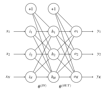
Regarding the topology of a MLP it is normally assumed to be a densely-meshed one-to-many link model between the layers. This is mathematically represented by two matrices of parameters named “the thetas”. In any case, if a certain connection is of little relevance with respect to the observable training data, the network will automatically pay little attention to its contribution and assign it a low weight close to zero.

Prediction

The evaluation of the output of a neural network, i.e., its prediction, given an input vector of data is a matter of matrix multiplication. To that end, the following variables are described for convenience:

  • is the dimension of the input layer.
  • is the dimension of the hidden layer.
  • is the dimension of the output layer.
  • is the dimension of the corpus (number of examples).

Given the variables above, the parameters of the network, i.e., the thetas matrices, are defined as follows:

The following sections describe the ordered steps that need to be followed in order to evaluate the network prediction.

Input Feature Expansion

The first step to attain a successful operation of the neural network is to add a bias term to the input feature space (mapped to the input layer):

The feature expansion of the input space with the bias term increases the learning effectiveness of the model because it adds a degree of freedom to the adaptation process. Note that directly represents the activation values of the input layer. Thus, the input layer is linear with the input vector (it is defined by a linear activation function).

Transit to the Hidden Layer

Once the activations (outputs) of the input layer are determined, their values flow into the hidden layer through the weights defined in :

Similarly, the dimensionality of the hidden layer is expanded with a bias term to increase its learning effectiveness:

Here, a new function is introduced. This is the generic activation function of a neuron, and generally it is non-linear, see below. Its application yields the output values of the hidden layer and provides the true learning power to the neural model.

Output Prediction

Finally, the activation values of the output layer, i.e., the network prediction, are calculated as follows:

Activation Function

The activation function of the neuron is a non-linear function that provides the expressive power to the neural network. Typically, the sigmoid function or the hyperbolic tangent function is used. It is recommended this function be smooth, differentiable and monotonically non-decreasing (for learning purposes).

Note that the range of these functions varies from to , respectively. Therefore, the output values of the neurons will always be bounded by the upper and the lower limits of these ranges. This entails considering a scaling process if a broader range of predicted values is needed.

Training

Training a neural network essentially means fitting its parameters to a set of example data considering an objective function, aka cost function. This process is also known as supervised learning. It is usually implemented as an iterative procedure.

Cost Function

The cost function somehow encodes the objective or goal that should be attained with the network. It is usually defined as a classification or a regression evaluation function. However, the actual form of the cost function is effectively the same, which is an error or fitting function.

The cost function quantifies the amount of error (or misfitting) that the network displays with respect to a set of data. Thus, in order to achieve a successfully working model, this cost function must be minimised with an adequate set of parameter values. To do so, several solutions are valid as long as this cost function be a convex function (i.e., a bowl-like shape). A well known example of such is the quadratic function, which trains the neural network considering a minimum squared error criterion over the whole dataset of training examples:

Note that the term in the cost function represents the target value of the network (i.e., the ideal/desired network output) for a given input data value . Now that the cost function can be expressed, a convex optimisation procedure (e.g., a gradient-based method) must be conducted in order to minimise its value. Note that this is essentially a least-squares regression.

One last remark should be made about the amount of examples . If the training procedure considers several instances at once per cost computation, i.e., , the approach is called batch learning. Batch learning is slow because each cost computation accounts for all the available training instances. In contrast, it is usual to consider only one training instance at a time, i.e., , in order to speed up the iterative learning process. This procedure is called online learning. Online learning steps are faster to compute, but this single-instance approximation of the cost function makes it a little inaccurate around the optimum. However, online learning is rather convenient in most cases.

Gradient Descent

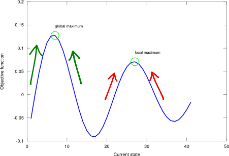
Given the convex shape of the cost function, the minimisation objective boils down to finding the extremum of this function. To this end you may use the analytic form of the derivative of the cost function (a nightmare), a numerical finite difference, or automatic differentiation.

Gradient descent is a first-order optimisation algorithm. It first starts with some arbitrarily chosen parameters and computes the derivative of the cost function with respect to each of them. The model parameters are then updated by moving them some distance (determined by the so called learning rate) from the former initial point in the direction of the steepest descent, i.e., along the negative of the gradient. These steps are iterated in a loop until some stopping criterion is met, e.g., a determined number of epochs (i.e., the single presentation of all patterns in the training example set) is reached.

Gradient descent is effectively the same algorithm as gradient ascent, but seeking a minimum of the objective function instead of a maximum. In order to reuse the already developed code (recall the DRY – Don’t Repeat Yourself principle, tip number 11 from The Pragmatic Programmer), I’m going to take the negative of the former cost function like in order to conduct the gradient descent approach with the gradient ascent algorithm. Note that the algorithm needs a learning rate parameter, which sets the step size used to update the neural network model parameters. If it is set too small, convergence is needlessly slow, whereas if it is too large, the update correction process may overshoot and even diverge.

Parameter Initialisation

The initial weights of the thetas assigned by the training process are critical with respect to the success of the learning strategy. They determine the starting point of the optimisation procedure, and depending on their value, the adjusted parameter values may end up in different places if the cost function has multiple (local) minima.

The parameter initialisation process is based on a uniform distribution between two small numbers that take into account the amount of input and output units of the adjacent layers:


In order to ensure a proper learning procedure, the weights of the parameters need to be randomly assigned in order to prevent any symmetry in the topology of the network model (that would be likely to incur convergence problems).

Regularisation

The mean squared-error cost function described above does not incorporate any knowledge or constraint about the characteristics of the parameters being adjusted through the gradient descent optimisation strategy. This may develop into a generalisation problem because the space of solutions is large and some of these solutions may turn the model unstable with new unseen data. Therefore, there is the need to smooth the performance of the model over a wide range of input data.

Neural networks usually generalise well as long as the weights are kept small. This tip is also in concordance with the parameter initialisation. Thus, the Tikhonov regularisation process, aka ridge regression, is introduced as a means to control complexity of the model in favour of its increased general performance. This regularisation approach favours small weight values:

There is a typical trade-off in Machine Learning, known as the bias-variance trade-off, which has a direct relationship with the complexity of the model, the nature of the data and the amount of available training data to adjust it. This ability of the model to learn more or less complex scenarios raises an issue with respect to its fitting: if the data is simple to explain, a complex model is said to overfit the data, causing its overall performance to drop (high variance model). Similarly, if complex data is tackled with a simple model, such model is said to underfit the data, also causing its overall performance to drop (high bias model). As it is usual in engineering, a compromise must be reached with an adequate value.

Practical Issues

The success of Artificial Intelligence and Machine Learning applications is plausibly conceived as a matter of controlling several key variables and following a series of “good practices”. There are some works in the literature that identify the bits and pieces to be taken into account when designing a successful model. Some of these are described as follows:

  • Focus on model generalisation: keep a separate self-validation set of data (not used to train the model) to test and estimate the actual performance of the model.
  • Incorporate as much knowledge as possible. Expertise is a key indicator of success. Data driven models don’t do magic, the more information that is available, the greater the performance of the model.
  • Feature Engineering is of utmost importance. This relates to the former point: the more useful information that can be extracted from the input data, the better performance can be expected. Salient indicators are keys to success. This may lead to selecting only the most informative features (mutual information, chi-square…), or to change the feature space that is used to represent the instance data (Principal Component Analysis…). And always standardise your data and exclude outliers.
  • Get more data if the model is not good enough. Related to “the curse of dimensionality” principle: if good data is lacking, no successful model can be obtained. There must be a coherent relation between the parameters of the model (i.e., its complexity) and the amount of available data to train them.
  • Ensemble models, integrate criteria. Bearing in mind that the optimum model structure is not known in advance, one of the most reasonable approaches to obtain a fairly good guess is to apply different models (with different learning features) to the same problem and combine/weight their outputs. Related techniques to this are also known as “boosting”.

The following sections delve into some of these topics with some practical strategies.

Target Values

When designing a learning system, it is suitable to take into account the nature of the problem at hand (e.g., whether if it is a classification problem or a regression problem) to determine the number of output units .

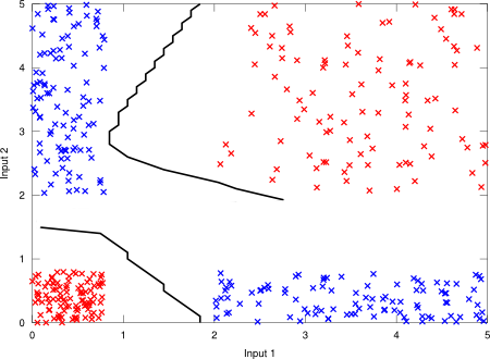
In the case of classification, should be the amount of different classes, and the target output should be a binary vector. Given an instance, only the output unit that corresponds to the instance class should be set. The decision rule for classification is then driven by the maximum output unit. Figure 2 shows a digital XOR gate with TTL technology (voltage thresholds are taken into account) with 2 inputs and 2  outputs (2 categories: “true” class or “false” class).

Figure 2. Digital XOR gate with TTL technology.

Digital XOR gate with TTL technology
Digital XOR gate with TTL technology.

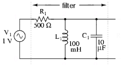
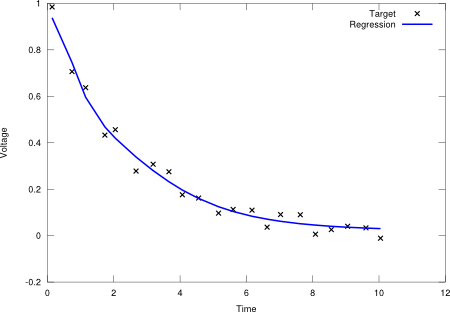
In the case of a regression problem, should be equal to the number of dependent variables. Figure 3 displays a regression over a capacitor discharge function (independent variable is time, dependent variable is voltage).

Figure 3. Capacitor discharge function.

Capacitor discharge function
Capacitor discharge function.

Hidden Units

The number of hidden units determines the expressive power of the network, and thus, the complexity of its transfer function. The more complex a model is, the more complicated data structures it can learn. Nevertheless, this argument cannot be extended ad infinitum because a shortage of training data with respect to the amount of parameters to be learnt may lead the model to overfit the data. That’s why the aforementioned regularisation function is used to avoid this situation.

Thus, it is common to have a skew toward suggesting a slightly more complex model than strictly necessary (regularisation will compensate for the extra complexity if necessary). Some heuristic guidelines to guess this optimum number of hidden units indicate an amount somewhat related to the number of input and output units. This is an experimental issue, though. There is no rule of thumb for this. Apply a configuration that works for your problem and you’re done.

The end

Presently, there is hype about deep learning (i.e., like a rebranding of multilayer neural networks) as the next big thing in Machine Learning and Artificial Intelligence. However, until very recently, it was very hard to publish something in the scientific community about neural networks. Now the fashion is back and neural nets seem to be the fanciest technique that ever existed, and all problems seem to be solvable, especially when the size of the network grows to huge numbers (this is the era of big data, right?).

Figure 4. Artificial Neural Network.

-- Artificial neural network class (multilayer perceptron model).
--
-- Activation function is assumed to be sigmoid.
-- Tikhonov regularisation is set to 1.

ann = {}

-- PRE:
-- IN - size of input layer (number).
-- HID - size of hidden layer (number).
-- OUT - size of output layer (number).
--
-- POST:
-- Returns an instance of an ANN (table).

function ann:new(IN, HID, OUT)
  local newann = {Lin = IN, Lhid = HID, Lout = OUT}
  self.__index = self
  setmetatable(newann, self)
  newann:initw()
  return newann
end

-- POST:
-- Initialises the model (the thetas).

function ann:initw()
  local epsilonIN = math.sqrt(6) / math.sqrt(self.Lin + self.Lhid)
  local epsilonOUT = math.sqrt(6) / math.sqrt(self.Lhid + self.Lout)
  --
  local function initmat(din, dout, value)
    math.randomseed(os.time())
    local mat = {}
    for i = 1, dout do
      local aux = {}
      for j = 1, din do
        table.insert(aux, ((math.random() - 0.5) / 0.5 ) * value)
      end
      table.insert(mat, aux)
    end
    return mat
  end
  --
  self.thetain = initmat(self.Lin + 1, self.Lhid, epsilonIN)
  self.thetaout = initmat(self.Lhid + 1, self.Lout, epsilonOUT)
end

-- PRE:
-- input - feat [1,N] vector (table).
--
-- POST:
-- Returns output [1,K] vector (table).

function ann:predict(input)
  local function matprod(m1, m2)
    local result = {}
    -- init
    for i = 1, #m1 do
      local row = {}
      for j = 1, #m2[1] do
        table.insert(row, 0)
      end
      table.insert(result, row)
    end
    -- multiply
    for i = 1, #m1 do
      for j = 1, #m2[1] do
        local prod = 0
        for k = 1, #m1[1] do
          prod = prod + m1[i][k] * m2[k][j]
        end
        result[i][j] = prod
      end
    end
    return result
  end
  --
  local function sigmoid(x)
    local y = 1 / (1 + math.exp(-x))
    return y
  end
  -- input must be a column [N,1] vector (table).
  -- step 1
  local aIN = {{1}}
  for i = 1, #input do
    table.insert(aIN, {input[i]})
  end
  -- step 2
  local zHID = matprod(self.thetain, aIN)
  local aHID = {{1}}
  for i = 1, #zHID do
    table.insert(aHID, {sigmoid(zHID[i][1])})
  end
  -- step 3
  local azOUT = matprod(self.thetaout, aHID)
  for i = 1, #azOUT do
    azOUT[i][1] = sigmoid(azOUT[i][1])
  end
  local flatOUT = {}
  for i = 1, #azOUT do
    table.insert(flatOUT, azOUT[i][1])
  end
  return flatOUT
end

-- PRE:
-- feat - list of example feature vectors (table).
-- targ - list of target value vectors (table).
--
-- POST:
-- Fits the neural network params to the given data.
-- Returns training error (number).

function ann:train(feat, targ)
  require("gradient_ascent")
  local function saveThetas()
    local thetas = {}
    -- theta in
    for i = 1, self.Lhid do
      for j = 1, (self.Lin + 1) do
        table.insert(thetas, self.thetain[i][j])
      end
    end
    -- theta out
    for i = 1, self.Lout do
      for j = 1, (self.Lhid + 1) do
        table.insert(thetas, self.thetaout[i][j])
      end
    end
    return thetas
  end
  local function loadThetas(thetas)
    -- theta in
    local index = 1
    for i = 1, self.Lhid do
      for j = 1, (self.Lin + 1) do
        self.thetain[i][j] = thetas[index]
        index = index + 1
      end
    end
    -- theta out
    for i = 1, self.Lout do
      for j = 1, (self.Lhid + 1) do
        self.thetaout[i][j] = thetas[index]
        index = index + 1
      end
    end
  end
  local function cost(thetas)
    local sqerr, pr
    local J = 0
    loadThetas(thetas)
    for m = 1, #feat do
      pr = self:predict(feat[m])
      sqerr = 0
      for k = 1, #pr do
        sqerr = sqerr + math.pow(targ[m][k] - pr[k], 2)
      end
      J = J + sqerr
    end
    J = J / #feat
    -- Regularisation
    local R = 0
    for i = 1, #self.thetain do
      for j = 2, #self.thetain[1] do
        R = R + math.pow(self.thetain[i][j], 2)
      end
    end
    for i = 1, #self.thetaout do
      for j = 2, #self.thetaout[1] do
        R = R + math.pow(self.thetaout[i][j], 2)
      end
    end
    R = R * (0.01 / (self.Lin*self.Lhid + self.Lhid*self.Lout))
    return -(J + R)
  end
  -- flatten thetas
  local flatTheta = saveThetas()
  gradient_ascent(cost, flatTheta, 1)
  -- deflat theta, restore model
  trerr = cost(flatTheta)
  loadThetas(flatTheta)
  -- return training err
  return trerr
end

Neural networks are inherently hard per se, as they’ve always been. Getting them to succeed on a wide range of problems is a challenging task, indeed. However, their basic form of operation is simple. In fact, it is as simple as that of a plain (least squares) regression with a sophisticated fitting function. The complete code listing is shown in Figure 4. Actually, there exists a myriad of techniques to deal with many details (for example, the renown backpropagation learning algorithm), but without loss of generality, they have been left out of the scope aimed at this post (the big picture of neural nets). You’ll be reading about them in a future post in due time. Stay tuned!

Gradient-based methods

The same principles that reign in local search methods for discrete spaces also apply to continuous spaces, i.e., start at some random place and take little steps toward the maximum. Taking into account that most real-world problems are continuous, it is no surprise that the literature on this topic is vast. For conventional, well-understood problems, a gradient-based technique may be the best approach you can take. It’s really worth it having a look at how they work!

Search objectives in continuous spaces are broadly described by real-valued smooth functions , i.e., twice differentiable functions. Then, the gradient/derivative of this objective function is a vector that gives the magnitude and direction of the steepest slope:

With this you can perform steepest-ascent hill climbing by updating the current state (initially random) according to the formula:

where is a small constant often called the “step size”, which determines the amount of contribution that the gradient has in the update process. Little by little, one step at a time, the algorithm will get to the maximum. However, having to calculate the gradient expression analytically by hand is a pain in the arse. Instead, you can compute an empirical gradient (i.e., numerically) by evaluating the response to small increments in each dimension/variable.

In order to see the gradient ascent algorithm in action, I will use a parallel LC resonant band-pass filter, see Figure 1.

Figure 1. Parallel LC resonant band-pass filter. Source: All About Circuits.

Parallel LC resonant band-pass filter
Parallel LC resonant band-pass filter.

The goal here is to find the band-pass frequency (a real number) of this filter. Recall that this is to be done numerically (the resonance of this circuit is well known to be , so at 159.15Hz for these component values: L=100mH, C=10uF). Thus, the magnitude of the transfer function of this filter is given as follows:

Note that is the magnitude of the impedance of the parallel LC circuit. The landscape plot of this function (that is the frequency domain) is shown in Figure 2. Note that this particular problem is somewhat tricky for gradient ascent, because the derivative increases as it approaches the maximum, so it may easily diverge during the update process (a really small step size is mandatory here). Other objective (convex) functions like the exponential error are expected to be more suitable because they are normally smoother around the extrema.

Figure 2. Gradient ascent applied on the magnitude function of a parallel LC resonant band-pass filter.

Gradient ascent applied on the magnitude function of a parallel LC resonant band-pass filter
Gradient ascent applied on the magnitude function of a parallel LC resonant band-pass filter.

Despite the high peakedness of the he objective function, the gradient ascent method is able to find the maximum in a breeze. The complete code listing is shown in Figure 3. Regarding its computational complexity, the space is bounded by the size of the variables vector, but the time depends on the specific shape of the landscape, the size of the step, etc.

Figure 3. Gradient ascent algorithm.

-- Gradient ascent algorithm.
--
-- PRE:
-- objfun - objective funciton to maximise (funciton).
-- var - variables, starting point vector (table).
-- step - step size (number).
--
-- POST:
-- Updates var with the max of objfun.
--
-- Loop while evaluation increases.

function gradient_ascent(objfun, var, step)
  local epsilon = 1e-4
  local feval = objfun(var)
  local grad = {}
  for i = 1, #var do
    table.insert(grad, 0)
  end
  local newvar = {}
  for i = 1, #var do
    table.insert(newvar, 0)
  end
  while (true) do
    local preveval = feval
    -- calc grad
    for i = 1, #var do
      local value = var[i]
      var[i] = value + epsilon
      local right = objfun(var)
      var[i] = value - epsilon
      local left = objfun(var)
      var[i] = value
      grad[i] = (right - left) / (2 * epsilon)
    end
    -- new var
    for i = 1, #var do
      newvar[i] = var[i] + step * grad[i]
    end
    -- eval
    feval = objfun(newvar)
    if (feval > preveval) then
      -- update var
      for i = 1, #var do
        var[i] = newvar[i]
      end
    else
      break
    end
  end
end

You must note, though, that this is a simple optimisation technique that works well if one single global extremum is present, but that more refined tweaks need to be applied if the objective function gets more complex. In the end, gradient ascent is complete but non-optimal. A typical and effective way to add robustness and speed up the process is to take as a time-dependent function (measured by the number of iterations in the loop) that settles the learning capability, pretty much like the simulated annealing algorithm. Other strategies take into account the momentum of the learning process in order to speed it up at times, in addition to avoiding local maxima. There is also the venerable Newton-Raphson algorithm, which makes use of the Hessian matrix (involving second derivatives) to optimise the learning path, although it can be somewhat tedious to run because it involves matrix inversion. This is all a rich and endless source of PhD topics.

Having a basic knowledge of such gradient-based methods, though, opens up a full range of possibilities, such as the use of Artificial Neural Networks (ANN). ANN’s are very fashion nowadays because of the disruption of deep learning. I know I’m being a little ahead of time with this technique, but it’s just so appealing to tackle so many problems that I can’t resist (note that an ANN is part of the A.I. Maker logo). In the next post, you’ll see how ANN’s can be easily learnt and deployed by directly applying gradient-based methods on complex functions. Stay tuned!

A closer look at problem state encoding in genetic algorithms through electronics

Encoding problem state information in a genetic algorithm (GA) is one of the most cumbersome aspects of its deployment. GA deals with binary vectors, so this is the format that you must comply to in order to find optimum solutions with this technique. And depending on which strategy you choose to do it, the solution of the search process may be different, and/or the GA algorithm may take more or less time (and/or space) to reach it. In order to display some of these issues, I will go through a complete example with an electronic circuit in this post. Specifically, the circuit under analysis will be a non-inverting amplifier built with an OP07 operational amplifier, see Figure 1. The goal of this discrete optimisation problem will be to find the optimum values of its two resistors Rf and Rg (over a finite set, so that they may be available in the store and the circuit be implementable) that maximise the symmetric excursion of a 1V peak input sinusoidal signal without clipping. Let’s synthesise this circuit with GA!

Figure 1. Schematic of a non-inverting amplifier. Source: Wikipedia.

Schematic of a non-inverting amplifier
Schematic of a non-inverting amplifier.

First step: encode each resistor value alone into a binary array. It is a good approach to represent the bits of an integer number, where the weight of each bit is directly related to a specific weight of the resistive spectrum, i.e., the most significant bits always correspond to high resistor values (and vice-versa), see Figure 2. I had also tried to follow the colour-based encoding that resistors display, i.e., like a mantissa and an exponent, but it’s been much of a failure, which I suspect is given by the non-linear relation between bit weight and resistance value. Note that you must still check that the represented number is within the accepted range of resistor values. Otherwise, discard it by assigning a bad fitness score so that it is likely to disappear during the evolution process. In this example, I’ll be using the 10% standard resistor values, from 10 ohm to 820k ohm (so, 60 different values in total, 6 bits).

Figure 2. Resistor value encoding and crossover.

Resistor value encoding and crossover
Resistor value encoding and crossover.

Next, encode the two resistor values in an array to create an initial population. To this end, append one resistor to the other to build an aggregate individual, like [Rf Rg], again see Figure 2. When having to combine them, the crossover point will keep the value of one resistor stable while evolving the other under improvement, which makes perfect sense.

Now, the output function of the non-inverting amplifier is given by:

and the fitness function used to evaluate the effectiveness of a solution is mainly driven by the inverse of the error of the symmetric excursion of (recall that greater scores are for better individuals):

Taking into account that with a power supply of 15V the OP07 saturates at about 12V, let’s fix the maximum symmetric excursion of the output to 20V (i.e., ) to avoid signal clipping. Having all that set, you’re ready to start optimising. Having a look at the fitness surface that the GA algorithm will deal with, see Figure 3, it shows that it will have a hard time dealing with so many extrema. Note that all maxima are located on a 9x slope line, which indicates that the solution must maintain a ratio of 9 between Rf and Rg. Also note that resistors placed on the lower end of the resistance range tend to be more stable and consume more power, while the ones placed on the higher end of the range draw less current but are more unstable. Since none of these considerations are included in the fitness function, the GA procedure may end on any of these local maxima, e.g, and , with a fitness score of .

Figure 3. Fitness surface plot.

Fitness surface plot
Fitness surface plot.

The performance of a brute-force exhaustive iterative search solution is taken for reference here, which has a computational complexity in time of , where is amount of possible resistor values (i.e., 60), and is the number of resistors in circuit (i.e., 2). This yields a search space of 3600 states. No matter how fancy GA’s may be, for such small search space, exhaustive linear search is much faster (it takes less than a second, while GA takes 5 secs). With 4 resistors, though, the search space is over 12M and the two approaches take about 10 secs. Over this bound, GA is able to perform better. Long are the days when engineers had to assemble the prototype circuits on a breadboard to optimise the numerical values of each of the components, see this video at 6:15.

The genetic algorithms

A genetic algorithm (GA) is a variant of stochastic beam search, which involves several search points/states concurrently (similar to the shotgun approach noted in the former post), and somehow combines their features according to their performance to generate better successor states. Thus, GA differs from former approaches like simulated annealing that only rely on the modification and evolution of a single state.

In GA, each search state, aka individual, encodes the problem information, usually as a binary array. GA begins with a set of randomly generated states, called the population. Then, it iterates over the chain of evolution for a determined number of rounds, see Figure 1, described as follows:

  1. Fitness evaluation: each state is scored wrt some effectiveness criterion (higher values for better states).
  2. Selection: states are randomly sampled with a specific probability according to their fitness value.
  3. Crossover: selected individuals are randomly shuffled or combined at a specific point.
  4. Mutation: child individuals may flip some of their bits (each one with independent probability).

Figure 1. Chain of evolution in genetic algorithms.

Chain of evolution in genetic algorithms
Chain of evolution in genetic algorithms.

The advantage with GA comes from the ability of crossover to combine large blocks of bits (i.e., state information) that have evolved independently to perform a specific useful function. However, the successful use and application of GA requires careful engineering of the state representation and its encoding (in addition to the more common optimisation parameters like the population size or the number of evolution rounds). This has a deep impact on the performance of the algorithm. Figure 2 shows an example objective landscape where the state-space number is represented as a binary array of 5 bits (unsigned integer).

Figure 2. Genetic algorithm applied on a one-dimensional state-space landscape described by an example objective function .

Genetic algorithm on a state-space landscape
Genetic algorithm on a state-space landscape.

GA belongs to a family of metaheuristics, which are algorithms designed to tackle ill-defined functions where a clear and definite objective is impossible to use. GA are adequate for black box search processes. Figure 3 implements the GA algorithm. Note how no explicit objective function is given. Instead, an initial population and a fitness function are passed to begin the search for the optimum.

Figure 3. Genetic algorithm.

-- Genetic algorithm.
--
-- PRE:
-- population - set of individuals (table).
-- fitness - evaluate individual (function).
--
-- POST:
-- solution - solution state (table).
--
-- Each individual (state) is a binary array.
-- Population is ordered from best to worst according to fitness. It
-- must be greater than one.
-- Fitness is normalised from 0 (bad) to 1 (good).

local function sort_population(population, fitness)
  local function comp(x, y)
    return (fitness(x) < fitness(y))
  end
  return table.sort(population, comp)
end

local function random_selection(population, fitness)
  local fit = {}
  local sumfit = 0
  for i = 1, #population do
    local fitIndi = fitness(population[i])
    table.insert(fit, fitIndi)
    sumfit = sumfit + fitIndi
  end
  fit[1] = fit[1] / sumfit
  for i = 2, #fit do
    fit[i] = fit[i] / sumfit + fit[i-1]
  end
  local x, y
  local rx = math.random()
  local ry = math.random()
  for i = 1, #fit do
    if (rx < fit[i]) then
      x = population[i]
      break
    end
  end
  for i = 1, #fit do
    if (ry < fit[i]) then
      y = population[i]
      break
    end
  end
  return x, y
end

local function reproduce(x, y)
  local point = math.floor(math.random() * #x) + 1
  local child = {}
  for i = 1, point do
    child[i] = x[i]
  end
  for i = point + 1, #x do
    child[i] = y[i]
  end
  return child
end

local function mutate(x)
  for i = 1, #x do
    if (math.random() < 0.1) then
      x[i] = math.abs(x[i] - 1)
    end
  end
end

function genetic_algorithm(population, fitness)
  local solution
  for epoch = 1, 100 do
    sort_population(population, fitness)
    local new_population = {}
    for i = 1, #population do
      local x, y = random_selection(population, fitness)
      local child = reproduce(x, y)
      if (math.random() < 0.05) then
        mutate(child)
      end
      table.insert(new_population, child)
    end
    population = new_population
  end
  return population[1]
end

The GA algorithm suggested in AIMA does not posit any similarity with real world reproductive systems, though. Is it reasonable to prevent inbreeding? In nature, close genetic relation results in disorders. Such issues are not discussed, but they don’t seem to have much of an impact for function optimisation purposes (in this particular case, mutation may add value here by creating a new individual).

Finally, regarding the computational complexities of GA, the space complexity is given by the number of individuals in the population , and the time complexity is given by the intermediate processes of the evolution chain. I guess one the critical points is ranking the individuals according to their fitness value for sampling. In the former implementation, Lua’s table.sort function (based on quicksort) is used. However, I would expect an overall for a tractable amount of instances. Depending on how fine you are with respect to your specific problem, several options may fit. Use your most sensible and plausible bound here (and test it!).

The simulated annealing algorithm

Simulated annealing (SA) is a local search method that combines the features of hill climbing (incomplete, effective) with the features of a random walk (complete, ineffective) in a way that yields both efficiency and completeness. The overall working principle is quite similar to hill climbing (to move upwards to the maximum), but now the short-term decisions of where to go next are stochastic. If a random choice improves the situation, it is always accepted. Otherwise, the SA algorithm accepts the “bad” move with a given transition probability. This probability decreases exponentially with the badness of the move, and a temperature factor, which allows doing such irrational moves only during a short period of time (recall that the transition is to a worse state). Empirically, though, it can be shown that under certain circumstances (i.e., with tailored parameters), this may favour leaving a local maximum for heading toward the optimum, see Figure 1. The probability associated to this turning action is called the Boltzmann factor, and quantifies the likelihood that a system transitions to a new energy state at a given temperature.

Figure 1. Simulated annealing applied on a one-dimensional state-space landscape described by an example objective function .

Simulated annealing on a state-space landscape
Simulated annealing on a state-space landscape.

The origin of the SA algorithm is found in the metallurgic tempering process, where high temperature is first applied to a metal to produce an atomic disorder, and then it is cooled down gradually in order to align the atoms and leave the system in a crystalline state. The analogy with the local search problem is that SA first allows lots of possibilities (high temperature) hoping to cover the optimum with greater chance, and then the system is brought to a stable state (low temperature) before it yields a solution result.

Figure 2. Simulated annealing algorithm.

-- Simulated annealing algorithm.
--
-- PRE:
-- problem - array of costs, index indicates state (table).
-- start - starting state index (number).
-- schedule - mapping from time to temperature (function).
--   It must end with zero.
--
-- POST:
-- solution - solution state (number).

function simulated_annealing(problem, start, schedule)
  local current = start
  local t = 0
  while (true) do
    t = t + 1
    local T = schedule(t)
    if (T == 0) then return current end
    local move = math.random()
    local successor = current
    if (move < 0.5) then
      if (current > 1) then
        successor = current - 1
      end
    else
      if (current < #problem) then
        successor = current + 1
      end
    end
    local delta = problem[successor] - problem[current]
    if (delta > 0) then
      current = successor
    else
      if (math.random() < math.exp(delta / T)) then
        current = successor
      end
    end
  end
end

SA is simple, iterative, stable, has good searching properties, and it is easily modifiable to accommodate other criteria (e.g., minimum instead of maximum), see Figure 2. Similar to hill climbing, SA has a unit space complexity and a linear time complexity given by the time the temperature decreases from an initial value to zero. However, SA is rather sensitive to its time-dependent temperature factor, which is given by the “schedule” function. The schedule trades off between exploration (high temperature, ability to make big changes) and exploitation (low temperature, ability to deepen into the local area). This operational flexibility is what makes the difference between SA and a plain hill climbing alternative. As an example, an exponential decay schedule function with time constant is shown in Figure 3.

Figure 3. Exponential decay schedule function.

Exponential decay schedule function
Exponential decay schedule function.

I conducted a test using the aforementioned schedule and the sinc landscape with 3 points on the following state-space locations: 10 (within global max area), 2 (also within global max area), and 20 (within local max area), and the result is that all these points converge to the global maximum. Go ahead and try it! Run the unit test script! The SA algorithm enables the search point close to the local max to leave that zone and move towards the optimum, and the other search points to reach the global and stay there (not jiggling as much as to leave the optimum point). Usually, tackling unknown problems entails having to deal with the uncertainty of solution reliability. In order to shed some light into this, a “shotgun” approach may be of help: run the SA procedure starting in lots of different places and look at the results from a more statistical perspective (where the majority of the solutions fall and what their values are).

Local search and the hill climbing algorithm

The scope of local search methods goes beyond the “classical” approach of seeking the shortest path to a goal state in an observable, deterministic, and discrete environment. In local search, the path is irrelevant. It operates on the current node only (with a complete-state formulation) rather than on multiple paths simultaneously (no frontier is involved).

Local search looks for the extrema of an objective function in a non-systematic way, but it is complete, as it always finds reasonable solutions if they exist. Thus, it is adequate for optimisation problems. However, it is only guaranteed to be optimal if one single (global) extremum exists. Otherwise, it will get stuck on any of the local extrema.

Hill climbing in detail

Hill climbing, aka steepest-ascent, is a greedy approach that operates in a loop that continually moves in the direction of increasing value, that is, uphill, until it reaches a “peak” (i.e., a maximum) where no neighbour shows a higher value, see Figure 1.

Figure 1. Hill climbing applied on a one-dimensional state-space landscape described by an example objective function .

Hill climbing on a state-space landscape
Hill climbing on a state-space landscape.

Hill climbing gets stuck at local maxima, plateaus and ridges. In case of failure (i.e., not reaching the global maximum), you may restart the process with a different initial value. Hill climbing displays a unit space complexity (i.e., the current state) and a linear time complexity (with respect to the number of neighbouring states). Figure 2 implements this algorithm on a one-dimensional state-space.

Figure 2. Hill climbing algorithm.

-- Hill climbing algorithm.
--
-- PRE:
-- problem - must be an array of costs, index indicates state (table).
-- start - must be the starting state index (number).
--
-- POST:
-- solution - is the solution state (number).


function hill_climbing(problem, start)
  local current = start
  local neighbour
  local change
  while (true) do
    if (current == 1) then
      neighbour, change = eval_right(problem, current)
    elseif (current == #problem) then
      neighbour, change = eval_left(problem, current)
    else
      neighbour, change = eval_left(problem, current)
      if (change == false) then
        neighbour, change = eval_right(problem, current)
      end
    end
    if (change) then
      current = neighbour
    else
      return current
    end
  end
end

function eval_left(problem, current)
  if (problem[current - 1] > problem[current]) then
    return current - 1, true
  else
    return current, false
  end
end

function eval_right(problem, current)
  if (problem[current + 1] > problem[current]) then
    return current + 1, true
  else
    return current, false
  end
end

Despite the (arguably) poor performance of hill climbing to find the global maximum, it is an intuitive algorithm that provides a lot of insight into the nature of the optimisation problems and a rule of thumb to solve them. The next posts will address this lack of skill and suggest more powerful optimisation routines. Stay tuned!