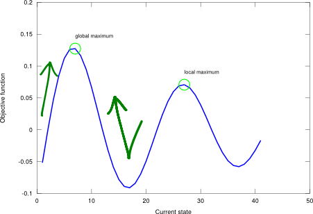
Simulated annealing (SA) is a local search method that combines the features of hill climbing (incomplete, effective) with the features of a random walk (complete, ineffective) in a way that yields both efficiency and completeness. The overall working principle is quite similar to hill climbing (to move upwards to the maximum), but now the short-term decisions of where to go next are stochastic. If a random choice improves the situation, it is always accepted. Otherwise, the SA algorithm accepts the “bad” move with a given transition probability. This probability decreases exponentially with the badness of the move, and a temperature factor, which allows doing such irrational moves only during a short period of time (recall that the transition is to a worse state). Empirically, though, it can be shown that under certain circumstances (i.e., with tailored parameters), this may favour leaving a local maximum for heading toward the optimum, see Figure 1. The probability associated to this turning action is called the Boltzmann factor, and quantifies the likelihood that a system transitions to a new energy state at a given temperature.

Figure 1. Simulated annealing applied on a one-dimensional state-space landscape described by an example objective function .

The origin of the SA algorithm is found in the metallurgic tempering process, where high temperature is first applied to a metal to produce an atomic disorder, and then it is cooled down gradually in order to align the atoms and leave the system in a crystalline state. The analogy with the local search problem is that SA first allows lots of possibilities (high temperature) hoping to cover the optimum with greater chance, and then the system is brought to a stable state (low temperature) before it yields a solution result.

Figure 2. Simulated annealing algorithm.

-- Simulated annealing algorithm.
--
-- PRE:
-- problem - array of costs, index indicates state (table).
-- start - starting state index (number).
-- schedule - mapping from time to temperature (function).
--   It must end with zero.
--
-- POST:
-- solution - solution state (number).

function simulated_annealing(problem, start, schedule)
  local current = start
  local t = 0
  while (true) do
    t = t + 1
    local T = schedule(t)
    if (T == 0) then return current end
    local move = math.random()
    local successor = current
    if (move < 0.5) then
      if (current > 1) then
        successor = current - 1
      end
    else
      if (current < #problem) then
        successor = current + 1
      end
    end
    local delta = problem[successor] - problem[current]
    if (delta > 0) then
      current = successor
    else
      if (math.random() < math.exp(delta / T)) then
        current = successor
      end
    end
  end
end

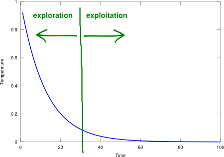
SA is simple, iterative, stable, has good searching properties, and it is easily modifiable to accommodate other criteria (e.g., minimum instead of maximum), see Figure 2. Similar to hill climbing, SA has a unit space complexity and a linear time complexity given by the time the temperature decreases from an initial value to zero. However, SA is rather sensitive to its time-dependent temperature factor, which is given by the “schedule” function. The schedule trades off between exploration (high temperature, ability to make big changes) and exploitation (low temperature, ability to deepen into the local area). This operational flexibility is what makes the difference between SA and a plain hill climbing alternative. As an example, an exponential decay schedule function with time constant is shown in Figure 3.

Figure 3. Exponential decay schedule function.

I conducted a test using the aforementioned schedule and the sinc landscape with 3 points on the following state-space locations: 10 (within global max area), 2 (also within global max area), and 20 (within local max area), and the result is that all these points converge to the global maximum. Go ahead and try it! Run the unit test script! The SA algorithm enables the search point close to the local max to leave that zone and move towards the optimum, and the other search points to reach the global and stay there (not jiggling as much as to leave the optimum point). Usually, tackling unknown problems entails having to deal with the uncertainty of solution reliability. In order to shed some light into this, a “shotgun” approach may be of help: run the SA procedure starting in lots of different places and look at the results from a more statistical perspective (where the majority of the solutions fall and what their values are).