Informed search, and the greedy search algorithm

Informed search strategies make use of problem-specific knowledge beyond the sole definition of the problem (i.e.,  the adjacency matrix of the graph), and take advantage of it to find solutions more efficiently than uninformed search strategies. The general informed search approach is called best-first search (BES). According to this method, a node must be selected for expansion based on an evaluation function (i.e., a cost estimate). In this sense, a heuristic function is the most common form to add knowledge into the BES algorithm. The heuristic indicates the estimated cost of the cheapest path from the present state to the goal state. Thus, the BES implementation is like uniform-cost search (UCS) but using a heuristic (node-wise vector) and an evaluation function (given as a handle) instead of the default accumulated path cost, see Figure 1.

Figure 1. Best-first search algorithm.

## @deftypefn {Function File} {@var{solution} =} best_first_search (@var{problem}, @var{start}, @var{finish}, @var{treegraph}, @var{feval}, @var{heuristic})
## Best-first search algorithm.
##
## PRE:
## @var{problem} must be the cost-weighted adjacency matrix.
## @var{start} must be the starting node index.
## @var{finish} must be the finishing node index.
## @var{treegraph} must be the tree/graph version flag. 0 is tree-version.
## @var{feval} must be a handle to the evaluation function.
## @var{heuristic} must be a heuristic at the node level.
##
## POST:
## @var{solution} is the solution path. State set to zero if failure.
##
## In this implementation, cost is a vector: [path_cost heuristic_cost].
## @end deftypefn

## Author: Alexandre Trilla <alex@atrilla.net>

function [solution] = best_first_search(problem, start, finish, ...
  treegraph, feval, heuristic)

  % inits
  node.state = start;
  node.parent = [];
  node.cost = [0 heuristic(start)];

  if (node.state == finish)
    solution = node;
  else
    frontier = [node];
    explored = [];
    found = 0;
    while (~found)
      if (numel(frontier) == 0)
        solution.state = 0;
        found = 1;
        break;
      endif
      % pop frontier, lowest cost node
      testNode = frontier(1);
      testIdx = 1;
      for i = 2:numel(frontier)
        if (feval(frontier(i).cost) < feval(testNode.cost))
          testNode = frontier(i);
          testIdx = i;
        endif
      endfor
      frontier = ...
        frontier([1:(testIdx-1) (testIdx+1):numel(frontier)]);
      node = testNode;
      % check
      if (node.state == finish)
        solution = node;
        break;
      endif
      % explore
      if (treegraph)
        explored(numel(explored)+1) = node.state;
      endif
      for i = 1:size(problem, 2)
        if (problem(node.state, i)>0)
          if (i ~= node.state)
            child.state = i;
            child.parent = [node.parent node.state];
            accumPath = node.cost(1) + problem(node.state, i);
            child.cost(1) = accumPath;
            child.cost(2) = heuristic(i);
            notExpl = 1;
            if (treegraph)
              notExpl = ~sum(explored == i);
            endif
            if (notExpl)
              inFront = 0;
              for j = 1:numel(frontier)
                if (frontier(j).state == i)
                  inFront = 1;
                  if (feval(frontier(j).cost) > feval(child.cost))
                    frontier(j) = child;
                  endif
                  break;
                endif
              endfor
              if (~inFront)
                frontier = [frontier child];
              endif
            endif
          endif
        endif
      endfor
    endwhile
  endif

endfunction

Note that the heuristic operates at the node level (not at the path level like a step cost). It’s a state fitness function and it doesn’t add-up over the traversal of nodes. With a good heuristic function, the complexity of the search procedure can be reduced substantially. The amount of the reduction, though, depends on the particular problem at hand and on the quality of the heuristic. And there is no free lunch here: developing a bespoke solution for a specific problem entails carefully designing a tailored heuristic, which generally works well only for this particular scenario.

A good heuristic never overestimates the number of steps to the solution. This requirement is commonly known as “admissibility”. In order to comply with it, the heuristic usually represents the cost of an optimal solution to a relaxed problem, which is the original problem without some constraints. Additionally, a heuristic may also show “consistency” if its estimated cost is monotonically non-increasing as it approaches the goal state (this is a stronger condition). As a rule of thumb, it is generally better to use a heuristic function with higher values provided it is consistent and that its computation is short.

Greedy search in detail

Greedy search (GS) is an informed search method that tries to expand the node that is strictly closest to the goal, assuming that it is likely to lead to a solution quickly. Thus, it evaluates neighbouring nodes by using only the heuristic function. Note that GS is not optimal nor complete (the immediate short-term benefit may not be the optimum one in the long run), but it is often efficient. Regarding its implementation, the former BES procedure is used with an anonymous evaluation function that returns the heuristic alone , see Figure 2.

Figure 2. Greedy search algorithm.

## @deftypefn {Function File} {@var{solution} =} greedy_search (@var{problem}, @var{start}, @var{finish}, @var{treegraph}, @var{heuristic})
## Greedy search algorithm.
##
## PRE:
## @var{problem} must be the cost-weighted adjacency matrix.
## @var{start} must be the starting node index.
## @var{finish} must be the finishing node index.
## @var{treegraph} must be the tree/graph version flag. 0 is tree-version.
## @var{heuristic} must be the heuristic vector.
##
## POST:
## @var{solution} is the solution path. State set to zero if failure.
## @end deftypefn

## Author: Alexandre Trilla <alex@atrilla.net>

function [solution] = greedy_search(problem, start, finish, treegraph,
  heuristic)

  % eval func is anonymous and returns heuristic
  solution = best_first_search(problem, start, finish, treegraph, ...
    @(cost) cost(2), heuristic);

endfunction

Following the UCS example with the graphical map of Germany, the heuristic of use for GS is based on the distance to München by motorways provided by ViaMichelin (a close resemblance to a straight-line distance). The resulting path from Frankfurt to München is the same, via Wurzburg and Nurnberg. However, GS resolves the problem in 6.96ms, while UCS does it in 12.4ms (almost double the time). Indeed, GS is more effective than UCS finding the best path in this informed environment.

The iterative deepening search algorithm

Iterative deepening search (IDS) combines the benefits of breadth-first and depth-first search: it has modest memory requirements (linear space complexity), and it is complete and optimal when the branching factor is finite, with a time complexity comparable to breadth-first ( is the depth of the solution). IDS works in tandem with depth-limited search and finds the best depth limit with a gradually increasing loop, see Figure 1. In general, IDS is the preferred uninformed search method when the search space is large and the depth of the solution is not known.

Figure 1. Iterative deepening search algorithm.

## @deftypefn {Function File} {@var{solution} =} iterative_deepening_search(@var{problem}, @var{start}, @var{finish})
## Iterative deepening search algorithm.
##
## PRE:
## @var{problem} must be the cost-weighted adjacency matrix.
## @var{start} must be the starting node index.
## @var{finish} must be the finishing node index.
##
## POST:
## @var{solution} is the solution path. State set to zero if there
## is no solution.
## @end deftypefn

## Author: Alexandre Trilla <alex@atrilla.net>

function [solution] = iterative_deepening_search(problem, start, ...
  finish)

  limit = 1;
  while (limit)
    solution = depth_limited_search(problem, start, finish, limit);
    limit += 1;
    if (solution.state ~= 1)
      break;
    endif
  endwhile

endfunction

With IDS you have got to the end of the section that deals with uninformed search strategies. What follows is the journey through informed search methods, where environment knowledge is incorporated in the search procedure in order to guide it (and thus make it more effective). Stay tuned!

The depth-limited search algorithm

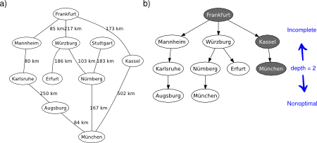
The depth-limited search (DLS) method is almost equal to depth-first search (DFS), but DLS solves the infinite state space problem because it bounds the depth of the search tree with a predetermined limit . Nodes at this depth limit are treated as if they had no successors. Thus, its time complexity is and its space complexity is ( is the branching factor). Note that DPS can be viewed as a special case of DLS with an infinite limit (in a sense, DLS is a more general approach). Also note that DLS is still incomplete (the given limit may be less than the depth of the solution) and nonoptimal (it may be greater), see Figure 1. However, in order to have an informed upper bound of the optimal depth limit, you can reasonably use the diameter of the state space (i.e., the longest shortest path between any two nodes defined by the problem).

Figure 1. DLS applied on the graphical map of Germany. Depth of solution from Frankfurt to München is 2. Source: Wikipedia. a) Problem description. b) Search tree.

DLS applied on the graphical map of Germany.
DLS applied on the graphical map of Germany

The tree search version of DLS can be conveniently implemented by exploiting recursivity, see Figure 2. The frontier is not explicitly declared but inherently maintained in the stack of calls.

Figure 2a. Depth-limited tree search algorithm.

## @deftypefn {Function File} {@var{solution} =} depth_limited_search (@var{problem}, @var{start}, @var{finish}, @var{limit})
## Recursive implementation of depth-limited tree search.
##
## PRE:
## @var{problem} must be the cost-weighted adjacency matrix.
## @var{start} must be the starting node index.
## @var{finish} must be the finishing node index.
## @var{limit} must be the depth limit.
##
## POST:
## @var{solution} is the solution path. Zero if standard failure
## (no solution). One if cutoff failure (no solution within the
## depth limit).
## @end deftypefn

## Author: Alexandre Trilla <alex@atrilla.net>

function [solution] = depth_limited_search(problem, start, ...
  finish, limit)

  node.state = start;
  node.parent = [];
  node.cost = 0;
  solution = recursive_dls(node, problem, finish, limit);

endfunction

Figure 2b. Recursive implementation of depth-limited tree search.

## @deftypefn {Function File} {@var{solution} =} recursive_dls(@var{node}, @var{problem}, @var{finish}, @var{limit})
## Recursive implementation of depth-limited tree search.
##
## PRE:
## @var{node} must be the starting node.
## @var{problem} must be the cost-weighted adjacency matrix.
## @var{finish} must be the finishing node index.
## @var{limit} must be the depth limit.
##
## POST:
## @var{solution} is the solution path. State set to zero if standard
## failure (no solution). One if cutoff failure (no solution within
## the depth limit).
## @end deftypefn

## Author: Alexandre Trilla <alex@atrilla.net>

function [solution] = recursive_dls(node, problem, finish, limit)

  if (node.state == finish)
    solution = node;
  elseif (limit == 0)
    solution.state = 1;
  else
    cutoff = 0;
    for i = 1:size(problem, 2)
      if (problem(node.state, i)>0)
        if (i ~= node.state)
          % expand search space
          child.state = i;
          path = node.parent;
          path = [path node.state];
          child.parent = path;
          child.cost = node.cost + problem(node.state, i);
          result = recursive_dls(child, problem, finish, ...
            limit - 1);
          if (result.state == 1)
            cutoff = 1;
          elseif (result.state ~= 0)
            solution = result;
            return;
          endif
        endif
      endif
    endfor
    if (cutoff)
      solution.state = 1;
    else
      solution.state = 0;
    endif
  endif

endfunction

Notice that DLS can terminate with two kinds of failure: the “no solution” standard failure, and the “cutoff” failure that indicates no solution within the given depth limit. In the next post, you are going to see how the accurate tracking of the given depth limit enables a DLS-inspired algorithm to be both complete and optimal. Stay tuned!

Depth-first search

Depth-first search (DFS) is a strategy that expands the deepest node in the current frontier. Thus, the frontier is based on a Last-In First-Out node container. The DFS approach is not optimal nor complete. The solution it yields is not based on any particular cost criterion: depending on which path is explored first the result may vary. Let’s say it is a somewhat “daring” approach because it takes the first path it comes across and goes to the end with it hoping it leads to the destination as soon as possible. This gives DFS a space complexity advantage over its breadth-first counterpart. While DFS has an equally concerning exponential time complexity , where is the branching factor and is the maximum depth of the search tree, it has a linear space complexity , which makes it more appealing for an effective (and feasible) implementation. DFS saves a lot of memory because it needs to store only one path from the root of the search tree to a leaf node.

In order to implement the DFS algorithm, let’s now reap the benefit of having coded the abstract data type (ADT) search procedure. Note that DFS can be easily specified if the ADT-search algorithm is given a handle to a function that manages the frontier as a stack, see Figure 1.

Figure 1. Stack insertion function.

## @deftypefn {Function File} {@var{insertion} =} ins_fifo(@var{frontier}, @var{node})
## Stack insertion.
##
## PRE:
## @var{frontier} must be a struct array for the frontier.
## @var{node} must be a struct for the node.
##
## POST:
## @var{insertion} is the extended frontier.
## @end deftypefn

## Author: Alexandre Trilla <alex@atrilla.net>

function [insertion] = ins_lifo(frontier, node)

  insertion = [node frontier];

endfunction

Are you wondering why all these search strategies have such a similar implementation pattern? Does all seem to be a matter of tweaking a line or two and giving it a new name? You are right. They don’t need to be so similar. In the following post you’ll see how DFS is implemented applying recursivity, for development convenience, and how its complexity features can also be bounded. Stay tuned!

Uniform-cost search

Uniform-cost search (UCS) is somewhat similar to breadth-first search (BFS), but this new approach seeks the minimum-cost path instead of the shallowest path. This is accomplished by using a priority queue (ordered by path cost) for the frontier, and an extra check in case a shorter path to a frontier state is discovered while traversing the graph, see Figure 1.

Figure 1. Uniform-cost search algorithm.

## @var{problem} must be the cost-weighted adjacency matrix.
## @var{start} must be the starting node index.
## @var{finish} must be the finishing node index.
## @var{treegraph} must be the tree/graph version flag. 0 is tree-version.
##
## POST:
## @var{solution} is the solution path. State set to zero if failure.
## @end deftypefn

## Author: Alexandre Trilla <alex@atrilla.net>

function [solution] = uniform_cost_search(problem, start, ...
  finish, treegraph)

  % inits
  node.state = start;
  node.parent = [];
  node.cost = 0;
  
  if (node.state == finish)
    solution = node;
  else
    frontier = [node];
    explored = [];
    found = 0;
    while (~found)
      if (numel(frontier) == 0)
        solution.state = 0;
        found = 1;
        break;
      endif
      % pop frontier, lowest cost node
      testNode = frontier(1);
      testIdx = 1;
      for i = 2:numel(frontier)
        if (frontier(i).cost < testNode.cost)
          testNode = frontier(i);
          testIdx = i;
          continue;
        endif
      endfor
      frontier = ...
        frontier([1:(testIdx-1) (testIdx+1):numel(frontier)]);
      node = testNode;
      % check
      if (node.state == finish)
        solution = node;
        break;
      endif
      % explore
      if (treegraph)
        explored(numel(explored)+1) = node.state;
      endif
      for i = 1:size(problem, 2)
        if (problem(node.state, i)>0)
          if (i ~= node.state)
            child.state = i;
            path = node.parent;
            path = [path node.state];
            child.parent = path;
            child.cost = node.cost + problem(node.state, i);
            notExpl = 1;
            if (treegraph)
              notExpl = ~sum(explored == i);
            endif
            if (notExpl)
              inFront = 0;
              for j = 1:numel(frontier)
                if (frontier(j).state == i)
                  inFront = 1;
                  if (frontier(j).cost > child.cost)
                    frontier(j) = child;
                  endif
                  break;
                endif
              endfor
              if (~inFront)
                frontier = [frontier child];
              endif
            endif
          endif
        endif
      endfor
    endwhile
  endif

endfunction

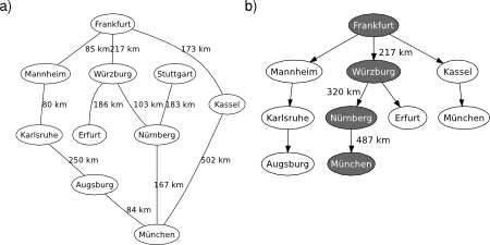
UCS is complete and optimal in general. Borrowing the same example from the Wikipedia, the shortest path (wrt distance) from Frankfurt to Münich is via Wüzburg and Nürnberg, which adds up to 487km (not 675km like the solution found via Kassel with BFS), see Figure 2.

Figure 2. UCS applied on the graphical map of Germany. Source: Wikipedia. a) Problem description. b) Search tree.

UCS applied on the graphical map of Germany.
UCS applied on the graphical map of Germany

Regarding its algorithmic complexity, UCS depends on path costs rather than on depths, so it is not easily characterised in terms of branching factor and depth of the solution (when all step costs are the same, UCS and BFS are pretty similar, i.e., they both have similar exponential complexities). However, since UCS is expected to explore all the nodes at the goal’s depth, it will usually do more work unnecessarily. In the following posts you’ll see how the completeness and optimality features can be relaxed to favour the algorithmic complexity of a search procedure. Stay up to date!

Refactoring breadth-first search

For the sake of generality, I have refactored the code of the breadth-first search (BFS) algorithm in order to accommodate both the tree and the graph-search versions. This has to do with the ability of the algorithm to deal with redundant paths, whether if they are to be taken into account (graph-search, as it is described in pseudocode in the book) or not (tree-search). The bulk of the code has been redefined as a generic abstract data type (ADT) search algorithm, which has an additional flag to use the explored set or not, see Figure 1 (changes are highlighted).

Figure 1. Abstract data type search algorithm.

## @deftypefn {Function File} {@var{solution} =} adt_search (@var{problem}, @var{start}, @var{finish}, @var{treegraph}, @var{insert})
## Abstract data type search algorithm.
##
## PRE:
## @var{problem} must be the cost-weighted adjacency matrix.
## @var{start} must be the starting node index.
## @var{finish} must be the finishing node index.
## @var{treegraph} must be the tree/graph version flag. Zero is
## tree-version.
## @var{insert} must be function handle to manage the insertion into
## the frontier.
##
## POST:
## @var{solution} is the solution path. State set to zero if failure.
## @end deftypefn

## Author: Alexandre Trilla <alex@atrilla.net>

function [solution] = adt_search(problem, start, ...
  finish, treegraph, insert)

  % inits
  node.state = start;
  node.parent = [];
  node.cost = 0;

  if (node.state == finish)
    solution = node;
  else
    frontier = [node];
    explored = [];
    found = 0;
    while (~found)
      if (numel(frontier) == 0)
        solution.state = 0;
        found = 1;
        break;
      endif
      % pop frontier
      node = frontier(1);
      frontier = frontier(2:end);
      % explore
      if (treegraph)
        explored(numel(explored)+1) = node.state;
      endif
      for i = 1:size(problem, 2)
        if (problem(node.state, i)>0)
          if (i ~= node.state)
            % by default, continue exploration
            notExpl = 1;
            if (treegraph)
              notExpl = ~sum(explored == i);
            endif
            if (notExpl)
              inFront = 0;
              for j = 1:numel(frontier)
                if (frontier(j).state == i)
                  inFront = 1;
                  break;
                endif
              endfor
              if (~inFront)
                % expand search space
                child.state = i;
                path = node.parent;
                path = [path node.state];
                child.parent = path;
                child.cost = node.cost + problem(node.state, i);
                % check goal
                if (i == finish)
                  solution = child;
                  found = 1;
                  break;
                else
                  frontier = insert(frontier,child);
                endif
              endif
            endif
          endif
        endif
      endfor
    endwhile
  endif

endfunction

Note that the ADT-search algorithm is also given a function handle to manage the insertion of a node into the frontier. The rationale for doing it is mainly to avoid the Don’t-Repeat-Yourself principle, i.e., the pragmatic programmer’s tip number 11. The benefit of this will come when we get to depth-first search. Stay tuned! Now, if this ADT-search algorithm is given a handle to a function that manages the frontier as a queue, see Figure 2, the functional behaviour of BFS remains the same.

Figure 2. Queue insertion function.

## @deftypefn {Function File} {@var{insertion} =} ins_fifo(@var{frontier}, @var{node})
## Queue insertion.
##
## PRE:
## @var{frontier} must be a struct array for the frontier.
## @var{node} must be a struct for the node.
##
## POST:
## @var{insertion} is the extended frontier.
## @end deftypefn

## Author: Alexandre Trilla <alex@atrilla.net>

function [insertion] = ins_fifo(frontier, node)

  insertion = [frontier node];

endfunction

A final note on the application scenario of BFS

The BFS algorithm (and in fact the rest of search routines you will see shortly) is to be deployed on environments that are deterministic, observable, static, and completely known. Otherwise, if the application scenario at hand does not display these characteristics, you simply can’t design an agent that performs actions to accomplish its goals with BFS.
BFS is a search strategy that seeks the shallowest path to the solution, it is complete (so it always finds a solution if there is one, at least), it is optimal for unit step costs, but it has exponential space complexity, which makes it infeasible for large-space search problems. Also note that the description of the search problem must be discrete, therefore the trees, graphs and their adjacency matrices. If continuous environments are to be searched with these methods, they must be discretised first, thus yielding a quantisation error according to the granularity of the grid of use. Or else use some common sense to reasonably represent the problem in discrete and tractable terms, like the BFS example with the map of Germany.

Breadth-first search

The first topic that is tackled in the AIMA book is problem solving by searching over a graphical structure. The overall operation of this family of algorithms is based on traversing the given graph, keeping unexplored nodes in a container called the “frontier”, and then exploring these nodes, one at a time. The strategy to conduct the search process, thus, depends on how nodes are managed with the frontier. If the frontier is treated as a queue, i.e., First-In First-Out, then the graph traversal is progressed via a breadth-first criterion, whereas if the frontier is used as a stack, i.e., Last-In First-Out, then the search algorithm expands by depth-first.

There is another issue regarding the redundancy of the paths. If the search algorithm does not take into account which nodes it explores along the way, it may traverse them more than once. This is called a tree-search algorithm. Instead, if it makes sure to not traverse the same node twice, it is called a graph-search algorithm. The suitability of one or the other depends on the nature of the objective problem at hand (and the ability of the searcher to trace its own footsteps in case it reaches a dead end).

Also, some search algorithms operate with the support of some guiding knowledge (that is like a kind of compass that points to the right direction), which are called informed search strategies, while others go around blindly without any knowledge at all about what next action is best, which are called uninformed search strategies. What must be common to all problem definitions, though, is that the step costs from one node to another be non-negative.

Based on the former premises, several search routines are typically defined. What follows are the details of the breadth-first search (BFS) algorithm.

BFS in detail

Breadth-first is an uninformed search strategy that seeks the shallowest path to the solution. Since it uses a FIFO queue for the frontier, the nodes at a given depth are always expanded before any nodes at the next level. This algorithm is commonly implemented following a graph-search template, see Figure 1, also available on the GitHub repository.

Figure 1. Breadth-first search algorithm.

## @deftypefn {Function File} {@var{solution} =} breadth_first_search (@var{problem}, @var{start}, @var{finish})
## Breadth-first search on a graph.
##
## PRE:
## @var{problem} must be the cost-weighted adjacency matrix.
## @var{start} must be the starting node index.
## @var{finish} must be the finishing node index.
##
## POST:
## @var{solution} is the solution path. State set to zero if failure.
## @end deftypefn

## Author: Alexandre Trilla <alex@atrilla.net>

function [solution] = breadth_first_search(problem, start, finish)

% inits
node.state = start;
node.parent = [];
node.cost = 0;

if (node.state == finish)
    solution = node;
else
    frontier = [node];
    explored = [];
    found = 0;
    while (~found)
        if (numel(frontier) == 0)
            solution.state = 0;
            found = 1;
            break;
        endif
        % pop frontier
        node = frontier(1);
        frontier = frontier(2:end);
        % explore
        explored(numel(explored)+1) = node.state;
        for i = 1:size(problem, 2)
            if (problem(node.state, i)>0)
                if (i ~= node.state)
                    if (~sum(explored == i))
                        inFront = 0;
                        for j = 1:numel(frontier)
                            if (frontier(j).state == i)
                                inFront = 1;
                                break;
                            endif
                        endfor
                        if (~inFront)
                            % expand search space
                            child.state = i;
                            path = node.parent;
                            path = [path node.state];
                            child.parent = path;
                            child.cost = node.cost + ...
                                problem(node.state, i);
                            % check goal
                            if (i == finish)
                                solution = child;
                                found = 1;
                                break;
                            else
                                frontier = [frontier child];
                            endif
                        endif
                    endif
                endif
            endif
        endfor
    endwhile
endif

endfunction

The gist of the BFS approach is to explore all possible options at a given point/level before making a decision on what to do next (i.e., the following node to be explored). Thus, it’s kind of hesitant. This has important implications on the computational complexity of this algorithm. Both time and space complexities are exponential with respect to the branching factor , i.e., the number of nodes that the search tree generates at a given level, and the depth of the solution: . Therefore, memory requirements are a bigger problem for BFS than is the execution time. In general, exponential-complexity search problems cannot be solved by uninformed methods for any but the smallest instances.

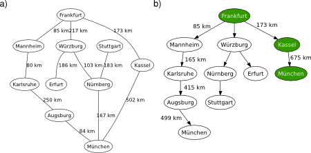
As a practical example, let’s use the graphical map of Germany from Wikipedia, see Figure 2a. If you apply BFS from Frankfurt to München, for example, the algorithm resolves the problem via Kassel, which is the shallowest path (two hops), see Figure 2b. This is fine. However, this is by no means the least costly solution as the distance amounts to 675km: it is not optimum in this distance-cost sense.

Figure 2. BFS applied on the graphical map of Germany. Source: Wikipedia. a) Problem description. b) Search tree.

BFS applied on the graphical map of Germany.
BFS applied on the graphical map of Germany

BFS may be somewhat misleading in this case because it treats physical dimensions as if they all weighed the same. But there is room for improvement here. So stay tuned for the next post. There you will deal with the optimum search strategy that accounts for the lowest-cost path to resolve the traversal of the graph.

Welcome

Today I decided to become a better engineer, especially in Artificial Intelligence (AI). And I’m determined to do something about it. I’m going to do deliberate practice in order to sharpen my technical and business skills, and eventually attain this goal. That’s why I’m starting this blog. Here I will scrutinise the contents of the AIMA book, from A to Z, implement its algorithms, and use them to reengineer commonplace intelligent systems, just for kicks. As it is commonly stated in the maker community: DIY cannot compete with commercial products, but it is very rewarding to learn and understand how things work by making them (and even get to make them a little better).

The big scope

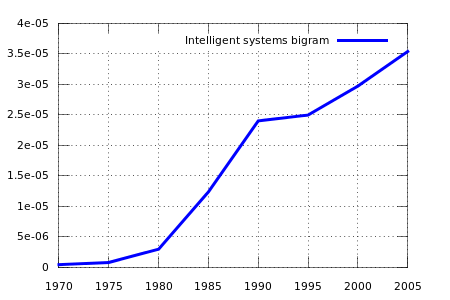
Borrowing the words from Paul Arden: it’s not how good you are, it’s how good you want to be. As a telecoms engineer with 10 years of professional experience, now helping companies leverage data to improve their competitiveness, I feel it’s time to compile all the knowledge I’ve gained over this time and do something awesome. It is also my goal to do so in the context of a healthy competitive business market. If intelligent systems are indeed in growing demand at present, e.g., see Figure 1 below, let’s discover the needs of the prospect customers and target them to drive future research. Pragmatic AI is so prevalent in the industry nowadays that there are many insights that will be of my interest to explore here.

Figure 1. Aggregate usage of the “intelligent systems” bigram in books (case-insensitive). Source: Google Ngram Viewer.

Aggregate usage of the “intelligent systems” bigram (case-insensitive). Source: Google Ngram Viewer.
Intelligent systems bigram in books

And the deep understanding of AI is not only relevant for the technical issues from the trenches, management is also in great benefit of this. In the end, suppliers are only as good as you are. Nobody else will do the magic but you. Thus, acing it as a project manager entails knowing first about the problem scope and how to tackle it appropriately.

The tools

In this journey through AI, the use of the AIMA book as a main guiding reference will be most necessary (among other relevant references). Its contents are broad, comprehensive, of general purpose, and written in plain words. Then, in order to bring its ideas to tangible code, Octave will be used for several good reasons (as an approach to using a Matlab-like syntax with open-source software). Primarily, I aim to evaluate algorithms, avoiding to get bogged down in the details of an “actual” programming language. Also, it is wise to program with a language close to the problem domain, i.e., the pragmatic programming tip number 17. And no matter how fancy would it be to code AIMA in Python, this has already been done by Peter Norvig (one of its authors). You already use Python extensively at work, don’t you? Thus, let’s approach this differently. My will is to add value here by implementing this with a clear data-analysis-driven scripting language that has not been considered yet (as far as I know).

Matlab is a great tool, there’s no doubt about that, don’t get me wrong. In fact, it’s one the first tools that experienced a most rapid growth wrt the number of users for its convenience. Given its wide reach, it is the numerical computing platform that rules in academia, in the corporate world, and also within the maker scene. Some say that you ought to adopt the best tools that money can buy to increase productivity. I cherish this piece of advice, especially for my professional development, but I’m not paying the license fee myself to do the same work I can do with Octave, nor I want Matworks to ever sue me if I use a pirate version of their beloved product. So let’s give it a shot with Octave! In the end, it can be seamlessly blended into Matlab. Andrew Ng did a great job to prove this with the Machine Learning class.

An appeal

Now, before I bring this first post to a close, let me just tell you that this is a most thrilling project for me, for the sake of knowledge, and that I’ll grind away at unravelling the details of such intelligent techniques, paying careful attention to detail. The only thing I ask of you is to give some feedback if you find this interesting. If you have similar personal deeds, please share them too! So feel free to collaborate, post your doubts, tips, quips, whatever. Everything is welcome. I’m eager to be of help if I can. Take it for a free consulting service as long as you openly discuss it here. On the downside, though, I’m afraid the posting rate won’t be much high or steady (perhaps @ai_maker is more adequate for such a more frequent usage), especially if experiments are to be conducted, but the fruitful discussions are another story. Enjoy.